
✅作者简介:热爱科研的Matlab仿真开发者,修心和技术同步精进,matlab项目合作可私信。
🍎个人主页:Matlab科研工作室
🍊个人信条:格物致知。
更多Matlab仿真内容点击👇
⛄ 内容介绍
在机械工程中,结构板的挠度是一个重要的参数,它描述了结构在受到外部载荷作用时的变形情况。对于受到压力载荷作用的结构板,计算其挠度是一个复杂的问题。然而,现代技术的发展使得我们能够利用偏微分方程工具箱 (TM)来解决这个问题。
偏微分方程工具箱 (TM)是一种基于数值计算的软件工具,它能够帮助工程师和科学家解决各种偏微分方程问题。通过将结构板的挠度问题建模为一个偏微分方程,我们可以利用偏微分方程工具箱 (TM)来计算结构板在受到压力载荷作用时的挠度。
首先,我们需要将结构板的几何形状和材料特性输入到偏微分方程工具箱 (TM)中。这些参数包括结构板的长度、宽度、厚度以及材料的弹性模量和泊松比。通过这些输入,我们可以建立一个适当的偏微分方程模型来描述结构板的挠度。
接下来,我们需要考虑结构板所受到的压力载荷。这可以通过输入载荷的大小和分布方式来实现。偏微分方程工具箱 (TM)可以根据这些载荷参数计算出结构板的受力情况,并将其作为偏微分方程模型的边界条件。
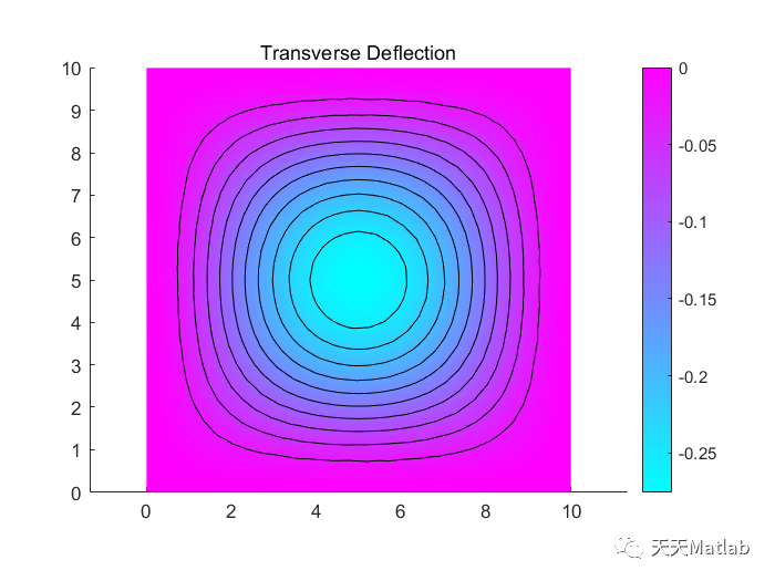
一旦我们完成了模型的建立和载荷的输入,偏微分方程工具箱 (TM)可以通过数值计算的方法求解这个偏微分方程模型。这将给出结构板在受到压力载荷作用时的挠度分布。我们可以通过可视化工具来显示这些结果,以便更好地理解结构板的变形情况。
使用偏微分方程工具箱 (TM)计算受压力载荷作用的结构板的挠度有许多优势。首先,它提供了一种准确和可靠的方法来解决这个复杂的问题。其次,偏微分方程工具箱 (TM)具有用户友好的界面,使得工程师和科学家能够轻松地使用它来进行计算。此外,它还可以处理各种不同类型的偏微分方程问题,使其具有广泛的适用性。
然而,使用偏微分方程工具箱 (TM)也存在一些挑战。首先,对于大型和复杂的结构板,计算时间可能会很长。此外,精确的模型参数和边界条件的选择也是一个关键问题,这需要工程师和科学家具备一定的专业知识和经验。
总之,基于偏微分方程工具箱 (TM)计算受压力载荷作用的结构板的挠度是一种强大而有效的方法。它为工程师和科学家提供了解决这个复杂问题的工具,并为他们提供了更深入地理解结构板变形行为的能力。随着技术的不断发展,我们相信偏微分方程工具箱 (TM)将在机械工程领域发挥越来越重要的作用。
⛄ 核心代码
%% Clamped, Square Isotropic Plate With a Uniform Pressure LoadThis example shows how to calculate the deflection of a structuralplate acted on by a pressure loadingusing the Partial Differential Equation Toolbox(TM).%% PDE and Boundary Conditions For A Thin PlateThe partial differential equation for a thin, isotropic plate with apressure loading is$$\nabla^2(D\nabla^2 w) = -p$$where $D$ is the bending stiffness of the plate given by$$ D = \frac{Eh^3}{12(1 - \nu^2)} $$and $E$ is the modulus of elasticity, $\nu$ is Poisson's ratio,and $h$ is the plate thickness. The transverse deflection of the plateis $w$ and $p$ is the pressure load.The boundary conditions for the clamped boundaries are $w=0$ and$w' = 0$ where $w'$ is the derivative of $w$ in a directionnormal to the boundary.The Partial Differential Equation Toolbox(TM) cannot directlysolve the fourth order plate equation shown above but this can beconverted to the following two second order partial differentialequations.$$ \nabla^2 w = v $$$$ D \nabla^2 v = -p $$where $v$ is a new dependent variable. However, it is not obvious how tospecify boundary conditions for this second order system. We cannotdirectly specify boundary conditions for both $w$ and $w'$.Instead, we directly prescribe $w'$ to be zero and use the followingtechnique to define $v'$ in such a way to insure that $w$ also equals zero onthe boundary. Stiff "springs"that apply a transverse shear force to the plate edge are distributedalong the boundary. The shear force along the boundary due to thesesprings can be written $n \cdot D \nabla v = -k w$ where $n$ is thenormal to the boundary and $k$ is the stiffness of the springs.The value of $k$ must be large enough that $w$ is approximately zeroat all points on the boundary but not so large that numerical errorsresult because the stiffness matrix is ill-conditioned.This expression is a generalized Neumann boundary condition supportedby Partial Differential Equation Toolbox(TM)In the Partial Differential Equation Toolbox(TM) definition for anelliptic system, the $w$ and $v$ dependent variables are u(1) and u(2).The two second order partial differential equations can be rewritten as$$ -\nabla^2 u_1 + u_2 = 0 $$$$ -D \nabla^2 u_2 = p $$which is the form supported by the toolbox. The input corresponding to thisformulation is shown in the sections below.%% Problem ParametersE = 1.0e6; % modulus of elasticitynu = .3; % Poisson's ratiothick = .1; % plate thicknesslen = 10.0; % side length for the square platehmax = len/20; % mesh size parameterD = E*thick^3/(12*(1 - nu^2));pres = 2; % external pressure%% Geometry and MeshFor a single square, the geometry and mesh are easily definedas shown below.gdmTrans = [3 4 0 len len 0 0 0 len len];sf = 'S1';nsmTrans = 'S1';g = decsg(gdmTrans', sf, nsmTrans');[p, e, t] = initmesh(g, 'Hmax', hmax);%% Boundary Conditionsb = @boundaryFileClampedPlate;type boundaryFileClampedPlate%% Coefficient DefinitionThe documentation for |assempde| shows the required formatsfor the a and c matrices in the section titled"PDE Coefficients for System Case". The most convenient form for cin this example is $n_c = 3N$ from the table where $N$ is the numberof differential equations. In this example $N=2$.The $c$ tensor, in the form of an $N \times N$ matrix of $2 \times 2$ submatricesis shown below.$$\left[\begin{array}{cc|cc}c(1) & c(2) & \cdot & \cdot \\\cdot & c(3) & \cdot & \cdot \\ \hline\cdot & \cdot & c(4) & c(5) \\\cdot & \cdot & \cdot & c(6)\end{array} \right]$$The six-row by one-column c matrix is defined below.The entries in the full $2 \times 2$ a matrix and the $2 \times 1$ f vectorfollow directly from the definition of thetwo-equation system shown above.c = [1; 0; 1; D; 0; D];a = [0; 0; 1; 0];f = [0; pres];%% Finite Element and Analytical SolutionsThe solution is calculated using the |assempde| function and thetransverse deflection is plotted using the |pdeplot| function. Forcomparison, the transverse deflection at the plate center is alsocalculated using an analytical solution to this problem.u = assempde(b,p,e,t,c,a,f);numNodes = size(p,2);pdeplot(p, e, t, 'xydata', u(1:numNodes), 'contour', 'on');title 'Transverse Deflection'numNodes = size(p,2);fprintf('Transverse deflection at plate center(PDE Toolbox)=%12.4e\n', min(u(1:numNodes,1)));compute analytical solutionwMax = -.0138*pres*len^4/(E*thick^3);fprintf('Transverse deflection at plate center(analytical)=%12.4e\n', wMax);displayEndOfDemoMessage(mfilename)
⛄ 运行结果
⛳️ 代码获取关注我
❤️部分理论引用网络文献,若有侵权联系博主删除
❤️ 关注我领取海量matlab电子书和数学建模资料
🍅 仿真咨询
1 各类智能优化算法改进及应用
生产调度、经济调度、装配线调度、充电优化、车间调度、发车优化、水库调度、三维装箱、物流选址、货位优化、公交排班优化、充电桩布局优化、车间布局优化、集装箱船配载优化、水泵组合优化、解医疗资源分配优化、设施布局优化、可视域基站和无人机选址优化
2 机器学习和深度学习方面
卷积神经网络(CNN)、LSTM、支持向量机(SVM)、最小二乘支持向量机(LSSVM)、极限学习机(ELM)、核极限学习机(KELM)、BP、RBF、宽度学习、DBN、RF、RBF、DELM、XGBOOST、TCN实现风电预测、光伏预测、电池寿命预测、辐射源识别、交通流预测、负荷预测、股价预测、PM2.5浓度预测、电池健康状态预测、水体光学参数反演、NLOS信号识别、地铁停车精准预测、变压器故障诊断
2.图像处理方面
图像识别、图像分割、图像检测、图像隐藏、图像配准、图像拼接、图像融合、图像增强、图像压缩感知
3 路径规划方面
旅行商问题(TSP)、车辆路径问题(VRP、MVRP、CVRP、VRPTW等)、无人机三维路径规划、无人机协同、无人机编队、机器人路径规划、栅格地图路径规划、多式联运运输问题、车辆协同无人机路径规划、天线线性阵列分布优化、车间布局优化
4 无人机应用方面
无人机路径规划、无人机控制、无人机编队、无人机协同、无人机任务分配
、无人机安全通信轨迹在线优化
5 无线传感器定位及布局方面
传感器部署优化、通信协议优化、路由优化、目标定位优化、Dv-Hop定位优化、Leach协议优化、WSN覆盖优化、组播优化、RSSI定位优化
6 信号处理方面
信号识别、信号加密、信号去噪、信号增强、雷达信号处理、信号水印嵌入提取、肌电信号、脑电信号、信号配时优化
7 电力系统方面
微电网优化、无功优化、配电网重构、储能配置
8 元胞自动机方面
交通流 人群疏散 病毒扩散 晶体生长 火灾扩散
9 雷达方面
卡尔曼滤波跟踪、航迹关联、航迹融合、状态估计
内容中包含的图片若涉及版权问题,请及时与我们联系删除

评论
沙发等你来抢