
✅作者简介:热爱科研的Matlab仿真开发者,修心和技术同步精进,matlab项目合作可私信。
🍎个人主页:Matlab科研工作室
🍊个人信条:格物致知。
更多Matlab完整代码及仿真定制内容点击👇
🔥 内容介绍
气泡饼图是数据可视化中一种独特而有趣的图表类型。它将饼图和散点图的特点结合在一起,通过展示数据的比例和分布情况,使得观察者能够更直观地理解数据背后的含义。在本文中,我们将深入探讨气泡饼图的特点、应用场景以及如何创建和解读这种图表。
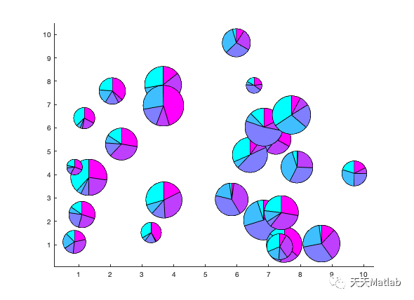
首先,让我们来了解一下气泡饼图的基本构成。与传统的饼图相比,气泡饼图在每个扇形区域内添加了一个气泡,气泡的大小代表了该区域所占比例的大小。这种设计使得气泡饼图能够同时展示数据的相对比例和绝对数值,提供了更全面的信息。
气泡饼图的应用场景非常广泛。首先,它常用于展示不同类别或组织之间的比例关系。例如,在市场调研中,我们可以使用气泡饼图来展示各个品牌的市场份额,气泡的大小代表了各个品牌的销售额。这样一来,我们可以直观地看到不同品牌之间的相对比例以及整个市场的规模。
此外,气泡饼图还可以用于展示多维数据之间的关系。例如,在人口统计学中,我们可以使用气泡饼图来展示不同年龄段的人口比例,气泡的大小可以表示该年龄段的人口数量。这样一来,我们可以通过观察气泡饼图,快速了解不同年龄段的人口分布情况。
在创建气泡饼图时,我们需要注意一些关键的步骤。首先,我们需要确定要展示的数据集,并将其按照比例转换为角度。然后,我们需要计算每个扇形区域的起始角度和结束角度。接下来,我们可以根据数据的绝对数值确定每个扇形区域内气泡的大小。最后,我们可以使用数据可视化工具或编程语言来创建气泡饼图,并添加必要的标签和图例,使得图表更易于理解和解读。
解读气泡饼图时,我们需要注意一些关键的要点。首先,我们应该关注气泡的大小,以了解不同区域所占比例的大小。其次,我们可以比较不同区域之间的气泡大小,以了解它们之间的相对比例。此外,我们还可以观察气泡的位置和分布情况,以获取更多关于数据的洞察。
总结一下,气泡饼图是一种独特而有趣的数据可视化工具,它能够同时展示数据的比例和分布情况。通过使用气泡饼图,我们可以更直观地理解数据背后的含义,并从中获取有价值的洞察。在今天数据驱动的世界中,气泡饼图无疑是一种强大的工具,帮助我们更好地理解和传达数据。无论是市场调研、人口统计学还是其他领域,气泡饼图都将成为我们分析和展示数据的重要利器。
📣 部分代码
BubbleChart ExamplesA BubblePie chart visualizing the revenue of an imaginary store that sells pizza ingredients.XData = 2015:2017;YData = [50 80 65];PieData = [12,26,12; 40,15,25; 10,10,45];b = bubblePieChart(XData, YData, PieData);b.LineStyle = 'none';b.Labels = {'Basil','Tomatoes','Cheese'};colororder([.47 .67 .19; .85 .33 .1; 1 1 .1]);xlabel("Year")ylabel("Revenue (thousands)")title("Pizza Ingredient Sales")A BubblePie chart plotting 25 pies with random data and sizes.XData = 10 * rand(1,25);YData = 10 * rand(1,25);PieData = rand(25,5);SizeData = 40 * rand(1,25) + 20;b = bubblePieChart(XData, YData, PieData, SizeData);colororder(cool(5));b.LegendVisible = 'off';
classdef bubblePieChart < matlab.graphics.chartcontainer.ChartContainer & ...matlab.graphics.chartcontainer.mixin.Legend% bubblePieChart Creates a bubble pie chart.% bubblePieChart(x,y,p) create a bubble pie chart with the specified% pie locations and data. The sizes of the pies are determined% automatically based on the pie data.%% bubblePieChart(x,y,p,s) create a bubble pie chart with% the specified size for each pie in points, where one point equals% 1/72 of an inch. s can be a scalar or a vector the same length as x% and y. If s is a scalar, the same size is used for all pies.%% bubblePieChart() create a bubble pie chart using only name-value% pairs.%% bubblePieChart(___,Name,Value) specifies additional options for% the bubble pie chart using one or more name-value pair arguments.% Specify the options after all other input arguments.%% bubblePieChart(parent,___) creates the bubble pie chart in the% specified parent.%% b = bubblePieChart(___) returns the bubblePieChart object. Use b% to modify properties of the plot after creating it.% Copyright 2020-2021 The MathWorks, Inc.properties% x-axis locations of the piesXData (1,:) = []% y-axis locations of the piesYData (1,:) = []% Pie data, specified as a matrix, where each row corresponds to% the data for one piePieData {mustBeNumeric} = []% Pie sizes, diameters in points (1/72 inch)SizeData (1,:) {mustBeNumeric} = 50% Line style to use for drawing piesLineStyle {mustBeMember(LineStyle,{'-', '--',':','-.','none'})} = '-'% Names of the pie categoriesLabels (:,1) categorical = categorical.empty(0,1)% Title of the plotTitle (:,1) string = ""% Subtitle of the plotSubtitle (:,1) string = ""% x-label of the plotXLabel (:,1) string = ""% y-label of the plotYLabel (:,1) string = ""% Mode for the x-limits.% Note that it is not a dependent property since auto limits are% set by the chart and not the axesXLimitsMode (1,:) char {mustBeAutoManual} = 'auto'% Mode for the y-limits.YLimitsMode (1,:) char {mustBeAutoManual} = 'auto'endproperties (Access = protected)% Used for saving to .fig filesChartState = []endproperties(Access = private,Transient,NonCopyable)% Array of parent transforms for the piesPieChartArray (1,:) matlab.graphics.primitive.Transform% Boolean specifying if PieData was changed since the previous call% to update. If true, all pies need to be redrawn.PieDataChanged logical = trueendproperties (Dependent)% List of colors to use for pie categoriesColorOrder {validatecolor(ColorOrder, 'multiple')} = get(groot, 'factoryAxesColorOrder')% x-limits of the plotXLimits (1,2) double {mustBeLimits} = [0 1]% y-limits of the plotYLimits (1,2) double {mustBeLimits} = [0 1]endmethodsfunction obj = bubblePieChart(varargin)% Initialize list of argumentsargs = varargin;leadingArgs = cell(0);% Check if the first input argument is a graphics object to use as parent.if ~isempty(args) && isa(args{1},'matlab.graphics.Graphics')% bubblePieChart(parent, ___)leadingArgs = args(1);args = args(2:end);end% Check for optional positional arguments.if ~isempty(args) && numel(args) >= 3 && isnumeric(args{1}) ...&& isnumeric(args{2}) && isnumeric(args{3})if mod(numel(args),2) == 1% bubblePieChart(x,y,p)% bubblePieChart(x,y,p,Name,Value)x = args{1};y = args{2};p = args{3};% set size automatically. The largest pie has size 50% and the others are scaled relative to ittotals = sum(p,2);ratios = totals/max(totals);s = 50*ratios;leadingArgs = [leadingArgs {'XData', x, 'YData', y, 'PieData', p, 'SizeData', s}];args = args(4:end);elseif mod(numel(args),1) == 0% bubblePieChart(x,y,p,s)% bubblePieChart(x,y,p,s,Name,Value)x = args{1};y = args{2};p = args{3};s = args{4};leadingArgs = [leadingArgs {'XData', x, 'YData', y, 'PieData', p, 'SizeData', s}];args = args(5:end);elseerror('bubblePieChart:InvalidSyntax', ...'Specify x locations, y locations, pie data, and optionally size data.');endend% Combine positional arguments with name/value pairs.args = [leadingArgs args];% Call superclass constructor methodobj@matlab.graphics.chartcontainer.ChartContainer(args{:});endendmethods(Access = protected)function setup(obj)% Create the axesax = getAxes(obj);ax.Units = 'points';% make limit mode manual so that we can control the limitsax.XLimMode = 'manual';ax.YLimMode = 'manual';% Set axes interactionsax.Interactions = [panInteraction;zoomInteraction;rulerPanInteraction];% Set restoreview button callbackbtn = axtoolbarbtn(axtoolbar(ax), 'icon', 'restoreview');btn.ButtonPushedFcn = @(~,~) update(obj);% Call the load method in case of loading from a fig fileloadstate(obj);endfunction update(obj)ax = getAxes(obj);% Verify that the data properties are consistent with one% another.showChart = verifyDataProperties(obj);set(obj.PieChartArray,'Visible', showChart);% Abort early if not visible due to invalid data.if ~showChartreturnend% If pie data is changed, delete and recreate all piesif obj.PieDataChangeddelete(obj.PieChartArray);hold(ax,'on');for r = 1:size(obj.PieData,1)% Create new Transformt = hgtransform('Parent',ax);obj.PieChartArray(r) = t;% Create new pie with transform as parentx = obj.PieData(r,:);myPie(t,x);endhold(ax,'off')obj.PieDataChanged = false;end% Set only the first pie chart to show in the legendobj.PieChartArray(1).Annotation.LegendInformation.IconDisplayStyle = 'children';% Update legend labelsif ~isempty(obj.Labels)lgd = getLegend(obj);lgd.String = obj.Labels;end% Set Colormap based on ColorOrderax.Colormap = obj.ColorOrder(mod(0:size(obj.PieData,2)-1,size(obj.ColorOrder,1))+1,:);% Automatically set axes limitsif strcmp(obj.XLimitsMode,'auto')obj.setAutoXLimits();endif strcmp(obj.YLimitsMode,'auto')obj.setAutoYLimits();end% Set position, scale, and style of each piefor i = 1:length(obj.PieChartArray)% move and scale piestxy = makehgtform('translate', ...[obj.XData(i), obj.YData(i), 0]);% Determine scale to use% divide by 2 since SizeData corresponds to diameter, and% default pies have radius of 1if isscalar(obj.SizeData)scale = obj.SizeData/2;elsescale = obj.SizeData(i)/2;end% Convert scale from axis units to data unitssx = (ax.XLim(2) - ax.XLim(1))*scale/ax.Position(3);sy = (ax.YLim(2) - ax.YLim(1))*scale/ax.Position(4);sxy = makehgtform('scale',[sx, sy, 1]);obj.PieChartArray(i).Matrix = txy * sxy;patches = findall(obj.PieChartArray(i), 'Type', 'Patch');set(patches,'LineStyle',obj.LineStyle);end% Set titletitle(ax, obj.Title, obj.Subtitle);% Set axis labelsxlabel(ax, obj.XLabel);ylabel(ax, obj.YLabel);endfunction showChart = verifyDataProperties(obj)% x and y must be the same length.showChart = numel(obj.XData) == numel(obj.YData);if ~showChartwarning('bubblePieChart:DataLengthMismatch',...'XData and YData must be the same legnth');returnend% PieData must have the same number of rows as the length of xshowChart = size(obj.PieData,1) == numel(obj.XData);if ~showChartwarning('bubblePieChart:DataLengthMismatch',...'PieData must have the same number of rows as XData.');returnend% SizeData must be a scalar or be the same length as xshowChart = isscalar(obj.SizeData) || numel(obj.SizeData) == numel(obj.XData);if ~showChartwarning('bubblePieChart:DataLengthMismatch',...'SizeData must be a scalar or have the same number of rows as XData.');returnendendendmethodsfunction data = get.ChartState(obj)% This method gets called when a .fig file is savedisLoadedStateAvailable = ~isempty(obj.ChartState);if isLoadedStateAvailabledata = obj.ChartState;elsedata = struct;ax = getAxes(obj);% Get axis limits only if mode is manual.if strcmp(ax.XLimMode,'manual')data.XLim = ax.XLim;endif strcmp(ax.YLimMode,'manual')data.YLim = ax.YLim;endendendfunction loadstate(obj)% Call this method from setup to handle loading of .fig filesdata=obj.ChartState;ax = getAxes(obj);% Look for states that changedif isfield(data, 'XLim')ax.XLim=data.XLim;endif isfield(data, 'YLim')ax.YLim=data.YLim;endendfunction set.PieData(obj,val)obj.PieData = val;obj.PieDataChanged = true;endfunction updateNow(obj)update(obj);endfunction set.ColorOrder(obj, map)ax = getAxes(obj);ax.ColorOrder = validatecolor(map, 'multiple');endfunction map = get.ColorOrder(obj)ax = getAxes(obj);map = ax.ColorOrder;end% xlim methodfunction varargout = xlim(obj,varargin)ax = getAxes(obj);[varargout{1:nargout}] = xlim(ax,varargin{:});end% ylim methodfunction varargout = ylim(obj,varargin)ax = getAxes(obj);[varargout{1:nargout}] = ylim(ax,varargin{:});end% set and get methods for XLimitsfunction set.XLimits(obj,xlm)ax = getAxes(obj);ax.XLim = xlm;endfunction xlm = get.XLimits(obj)ax = getAxes(obj);xlm = ax.XLim;end% set and get methods for YLimitsfunction set.YLimits(obj,ylm)ax = getAxes(obj);ax.YLim = ylm;endfunction ylm = get.YLimits(obj)ax = getAxes(obj);ylm = ax.YLim;endendmethods(Access=private)% Helper function for auotmatically setting x-limitsfunction setAutoXLimits(obj)ax = getAxes(obj);minX = min(obj.XData);maxX = max(obj.XData);if(minX==maxX)minX = minX-1;maxX = maxX+1;endmaxRadius = min(max(obj.SizeData)/2, ax.Position(3)/3);A = [-maxRadius+ax.Position(3) maxRadius;maxRadius ax.Position(3)-maxRadius];b = [minX*ax.Position(3); maxX*ax.Position(3)];xlimits = A\b;obj.XLimits = xlimits;end% Helper function for auotmatically setting y-limitsfunction setAutoYLimits(obj)ax = getAxes(obj);minY = min(obj.YData);maxY = max(obj.YData);if(minY==maxY)minY = minY-1;maxY = maxY+1;endmaxRadius = min(max(obj.SizeData)/2, ax.Position(4)/3);A = [-maxRadius+ax.Position(4) maxRadius;maxRadius ax.Position(4)-maxRadius];b = [minY*ax.Position(4); maxY*ax.Position(4)];ylimits = A\b;obj.YLimits = ylimits;endendendfunction mustBeLimits(a)if numel(a) ~= 2 || a(2) <= a(1)throwAsCaller(MException('densityScatterChart:InvalidLimits', 'Specify limits as two increasing values.'))endendfunction mustBeAutoManual(mode)mustBeMember(mode, {'auto','manual'})end% Helper function for creating pies baesd on MATLAB's pie functionfunction h = myPie(ax,x)% Normalize input datax = x/sum(x);h = [];theta0 = pi/2;maxpts = 100;for i=1:length(x)n = max(1,ceil(maxpts*x(i)));r = [0;ones(n+1,1);0];theta = theta0 + [0;x(i)*(0:n)'/n;0]*2*pi;[xx,yy] = pol2cart(theta,r);theta0 = max(theta);h = [h,...patch('XData',xx,'YData',yy,'CData',i*ones(size(xx)), ...'FaceColor','Flat','parent',ax)]; %#ok<AGROW>endend
⛳️ 运行结果
🔗 参考文献
[1] 张蕾.基于神经网络的地区配变重过载预测研究[J].陕西理工大学, 2019.
[2] 俞建荣,卜凡亮,曹建树,等.基于Matlab的流化床气泡运动的图像识别与处理[J].仪器仪表学报, 2006(z3):2.DOI:10.3321/j.issn:0254-3087.2006.z3.215.
[3] 王寻,王宏哲,张泽坤,等.基于Matlab GUI的气泡动力学仿真系统设计[J].实验室研究与探索, 2022(004):041.
🎈 部分理论引用网络文献,若有侵权联系博主删除
🎁 关注我领取海量matlab电子书和数学建模资料
👇 私信完整代码和数据获取及论文数模仿真定制
1 各类智能优化算法改进及应用
生产调度、经济调度、装配线调度、充电优化、车间调度、发车优化、水库调度、三维装箱、物流选址、货位优化、公交排班优化、充电桩布局优化、车间布局优化、集装箱船配载优化、水泵组合优化、解医疗资源分配优化、设施布局优化、可视域基站和无人机选址优化
2 机器学习和深度学习方面
卷积神经网络(CNN)、LSTM、支持向量机(SVM)、最小二乘支持向量机(LSSVM)、极限学习机(ELM)、核极限学习机(KELM)、BP、RBF、宽度学习、DBN、RF、RBF、DELM、XGBOOST、TCN实现风电预测、光伏预测、电池寿命预测、辐射源识别、交通流预测、负荷预测、股价预测、PM2.5浓度预测、电池健康状态预测、水体光学参数反演、NLOS信号识别、地铁停车精准预测、变压器故障诊断
2.图像处理方面
图像识别、图像分割、图像检测、图像隐藏、图像配准、图像拼接、图像融合、图像增强、图像压缩感知
3 路径规划方面
旅行商问题(TSP)、车辆路径问题(VRP、MVRP、CVRP、VRPTW等)、无人机三维路径规划、无人机协同、无人机编队、机器人路径规划、栅格地图路径规划、多式联运运输问题、车辆协同无人机路径规划、天线线性阵列分布优化、车间布局优化
4 无人机应用方面
无人机路径规划、无人机控制、无人机编队、无人机协同、无人机任务分配、无人机安全通信轨迹在线优化
5 无线传感器定位及布局方面
传感器部署优化、通信协议优化、路由优化、目标定位优化、Dv-Hop定位优化、Leach协议优化、WSN覆盖优化、组播优化、RSSI定位优化
6 信号处理方面
信号识别、信号加密、信号去噪、信号增强、雷达信号处理、信号水印嵌入提取、肌电信号、脑电信号、信号配时优化
7 电力系统方面
微电网优化、无功优化、配电网重构、储能配置
8 元胞自动机方面
交通流 人群疏散 病毒扩散 晶体生长
9 雷达方面
卡尔曼滤波跟踪、航迹关联、航迹融合
内容中包含的图片若涉及版权问题,请及时与我们联系删除

评论
沙发等你来抢