
Stanford CS224W: Machine Learning with Graphs
By Avinash Rajput as part of the Stanford CS 224W Final Project
https://drive.google.com/file/d/14R0Y23KYfyBejO5HxWOET-69Ac8UNHzn/view?usp=sharing

Task Description and Motivation
任务描述和动机
In an era where medical knowledge advances at an increasing pace, theMednet serves as a bridge between textbooks and the nuanced complexities of real-world clinical practice. It is a simple truth that patients with access to experts have better outcomes. By capturing and then systematizing undocumented clinical insights, the platform ensures this expertise is accessible and easily searchable, empowering physicians to provide their patients with a high standard of care no matter where they are.
在医学知识不断进步的时代,Mednet 成为了教科书与真实世界临床实践复杂性的桥梁。一个简单的真理是,有专家可访问的患者会有更好的结果。通过捕捉并系统化未记录的临床洞察,该平台确保这种专业知识易于访问和搜索,使医生无论身在何处都能为患者提供高标准的服务。
Some background — theMednet operates as a platform exclusively for physicians, facilitating expert-driven discussions and answers to the complex challenges of real-world clinical practice. theMednet aims to serve as a nexus for nuanced medical inquiries/questions that often lie beyond the scope of textbooks or established guidelines. These questions delve deeply into specialized fields such as oncology, neurology, and rheumatology, reflecting the dynamic, evolving nature of medical care. By fostering collaborative exchanges among doctors, the platform enhances decision-making for complex cases, helping physicians deliver more precise and effective treatments. Ultimately, theMednet’s mission is to improve patient outcomes by equipping physicians with timely, practical, and evidence-informed guidance that they would not have access to otherwise. [1]
一些背景信息——Mednet 作为一个仅面向医生的平台,促进专家驱动的讨论和回答现实临床实践中复杂挑战的解决方案。Mednet 旨在成为深入医学探究/问题的枢纽,这些问题通常超出了教科书或现有指南的范围。这些问题深入到如肿瘤学、神经病学和风湿病学等专门领域,反映了医疗保健的动态、演变性质。通过促进医生之间的协作交流,该平台增强了复杂病例的决策能力,帮助医生提供更精确和有效的治疗方案。最终,Mednet 的使命是通过为医生提供及时、实用和基于证据的指导,从而改善患者预后,这些指导是他们否则无法获得的。[1]
To illustrate, consider a common use case: a physician treating a rare subtype of cancer submits a question regarding the latest advancements in treatment protocols for a patient with a secondary condition. Soon, responses from oncology experts — grounded in their firsthand experience and supported by emerging science — are shared on the platform. While this process effectively provides life-saving insights, it also highlights a key challenge: the need to ensure that the right questions reach the most relevant experts efficiently. This forms the foundation of our exploration — developing a predictive framework that connects questions to the physicians most likely to engage, thereby optimizing the flow of critical knowledge within theMednet ecosystem.
为了说明,考虑一个常见的用例:一位治疗罕见癌症亚型的医生提交了一个关于患有继发性疾病的患者最新治疗方案的提问。很快,来自肿瘤学专家的回答——基于他们的亲身经验和新兴科学的支持——在该平台上共享。虽然这个过程有效地提供了救命的知识,但也突显了一个关键挑战:确保正确的问题能够高效地到达最相关的专家。这构成了我们探索的基础——开发一个将问题与最有可能参与的医生相连接的预测框架,从而优化 Mednet 生态系统中的关键知识流动。
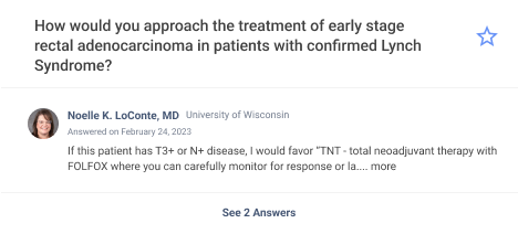
For reference, an example of a question from theMednet can be seen below:
以下是一个来自 Mednet 的提问示例,仅供参考:
As touched on above, we need to be able to show questions to doctors who can make the most of the information. This accomplishes two goals:
如上所述,我们需要能够向能够充分利用信息的医生展示问题。这实现了两个目标:
It provides answers to doctors who may find the question relevant to their practice
这为可能觉得问题与他们的实践相关的医生提供答案
It enables doctors with relevant knowledge to provide helpful answers to these life-changing questions
这使得拥有相关知识的医生能够为这些改变生命的问题提供有价值的答案
Therefore, the primary goal of this project is to predict the questions that a doctor is most likely to view. The secondary goal of this project is to predict the questions that a doctor is most likely to answer. Question-answer relations are a subset of question-view relations. We are highlighting this relationship because it was significant in the design of our models.
因此,本项目的首要目标是预测医生最有可能查看的问题。本项目的次要目标是预测医生最有可能回答的问题。问答关系是问答关系的子集。我们强调这种关系,因为它在我们的模型设计中具有重要意义。
The primary evaluation metrics for this project are Precision@K (proportion of recommendations that users interacted with) and Recall@K (proportion of interactions that had successful recommendations), for both question views and question answers. While we place a stronger emphasis on achieving high Precision@K — making sure the top K recommendations are highly relevant — we also want to maintain strong Recall@K. As we increase K, we want to ensure we are capturing the full range of relevant questions, not just the most obvious ones.
本项目的首要评估指标是 Precision@K(用户互动的推荐比例)和 Recall@K(成功推荐的互动比例),针对问题查看和问题回答。虽然我们更重视实现高 Precision@K——确保前 K 个推荐高度相关——但我们也希望保持强大的 Recall@K。随着 K 的增加,我们希望确保我们能够捕捉到所有相关问题的全范围,而不仅仅是显而易见的问题。
数据
数据来源和特征
Our graph is composed of Doctors and Questions as nodes. We construct feature vectors for the doctors based on their specialty, subspecialty, and activity statuses. We construct feature vectors for the questions based on their topic, author, publication status, and author anonymity.
我们的图由医生和问题作为节点组成。我们根据医生的专业、亚专业和活动状态构建医生的特征向量。我们根据问题的主题、作者、发布状态和作者匿名性构建问题的特征向量。
As we’ll see later, some models struggled to learn significant differences in the embeddings within questions and within doctors, making it difficult to differentiate individual data points. In order to counter this, we also randomly added a feature vector based on LLM returned keywords for a random sampling of 3% of the questions. This added some differentiating information about some of the questions, which we had hoped would inform the question embedding space. While it led to decreased cosine similarity in some models, it did not ultimately lead to improved achievement of project goals.
如我们稍后所见,一些模型在学习和区分问题和医生嵌入中的显著差异方面存在困难,这使得区分个别数据点变得困难。为了解决这个问题,我们还随机添加了一个基于LLM返回的关键词的特征向量,用于随机抽取的 3%的问题。这为一些问题添加了一些区分信息,我们希望这些信息能够告知问题嵌入空间。虽然这导致某些模型中的余弦相似度降低,但最终并没有导致项目目标的实现得到改善。
We focus on two primary relations: the question-view relation and the question-answer relation. There were other relations available to leverage, including connections between publications and doctors, publications and users, and other user activities such as asking and commenting on questions.
我们关注两个主要关系:问题-视图关系和问题-答案关系。还有其他可以利用的关系,包括出版物与医生、出版物与用户之间的联系,以及其他用户活动,如提问和评论问题。
数据预处理
We fixed the timespan of the dataset for consistency of analysis. The set included more than 20k questions, 254k users, and ~1 million publications. Depending on the model, we then create the various edge and relation types, which were around 7.8 million for the most expansive R-GCN model and roughly 6 million for the more focused GraphSage model.
我们为了分析的连贯性,固定了数据集的时间跨度。该集合包括超过 20k 个问题,254k 个用户和约 100 万篇出版物。然后根据模型,我们创建了各种边和关系类型,对于最广泛的 R-GCN 模型来说,大约有 780 万,而对于更专注的 GraphSage 模型来说,大约有 600 万。
The specialty, subspecialty, topics, and LLM generated features were one hot encoded and appended to the relevant feature matrices. The user, question, and publication feature matrices (where applicable) were then standardized to ensure they had the same dimensions.
将专业、亚专业、主题和LLM生成的特征进行独热编码,并附加到相关的特征矩阵中。然后对用户、问题和出版物特征矩阵(如有适用)进行标准化,以确保它们具有相同的维度。
The overall data set was split into 70% training, 15% validation, and 15% testing. For GraphSage models, negative samples were created using PyG’s negative_sample utility and assigned a no-edge label. For these models, negative samples were generated in a 1:1 ratio with positive samples. When executing recommendation/ranking focused tasks on R-GCNs, for negative samples, triplets were created by -
整个数据集被分为 70%的训练集、15%的验证集和 15%的测试集。对于 GraphSage 模型,使用 PyG 的 negative_sample 工具创建了负样本,并分配了无边标签。对于这些模型,负样本与正样本以 1:1 的比例生成。在执行针对 R-GCNs 的推荐/排序任务时,对于负样本,通过以下方式创建三元组:-
having a question as an anchor node,
以问题作为锚节点,
a user matching the edge type of focus as a positive node,
一个与焦点边类型匹配的用户作为正节点,
and a randomly selected user that did not have that edge type as a negative node.
以及随机选择的一个没有该边类型的用户作为负节点。
The triplet loss was computed with the following equation:
三元组损失的计算公式如下:

This encourages the model to learn embeddings where positive pairs have higher similarity than negative pairs by at least the margin amount.
这鼓励模型学习嵌入,使得正样本对之间的相似度至少比负样本对高 margin 值。
The number of samples generated were in ratio to the number of epochs and the number of edges. That is, the goal was to select enough triples per epoch such that we could expect that each edge would get sampled once over the course of the training. This made the goal for the number of triples sampled approximately equal to the number of edges divided by epochs. Because R-GCN was more computationally intensive it was sometimes not possible to do this with the Colab infrastructure. When executing edge classification tasks on R-GCNs, the negative samples were created by randomly finding nodes with no connections and assigning them edge class 0 (no edge). These were assigned in equal numbers to the positive edges for balance.
生成的样本数量与 epoch 数和边的数量成比例。也就是说,目标是每个 epoch 选择足够的三元组,以便我们预计每个边在整个训练过程中都会被采样一次。这使得采样三元组的数量大约等于边的数量除以 epoch 数。由于 R-GCN 计算量更大,有时在 Colab 基础设施上无法做到这一点。在执行 R-GCN 的边分类任务时,负样本是通过随机找到没有连接的节点并分配边类别 0(无边)来创建的。这些样本以平衡的方式分配给正边。
解释模型
Medical knowledge and physician interests do not exist in isolation. They are organized in interconnected patterns; doctors of certain subspecialties often engage with similar sets of questions — and certain types of questions attract doctors with related backgrounds. By placing physicians and questions in a shared graph structured space, GNNs (Graph Neural Networks) can learn these patterns in order to provide information to the doctors who need them the most. GNNs can also learn complex patterns between nodes and edges that traditional methods cannot capture. GNNs do this by passing messages between nodes across edges, aggregating the received information, and then updating features and weights. This process repeats across layers, allowing us to capture information from seemingly disparate nodes and clusters of nodes. This generally motivated the usage of GNNs for this problem.
医学知识和医生兴趣并非孤立存在。它们以相互关联的模式组织;某些专科的医生经常涉及相似的问题集——某些类型的问题会吸引具有相关背景的医生。通过将医生和问题放置在共享的图结构空间中,GNN(图神经网络)可以学习这些模式,以便为最需要的医生提供信息。GNN 还可以学习节点和边之间的复杂模式,这是传统方法无法捕捉的。GNN 通过在节点之间通过边传递消息,汇总接收到的信息,然后更新特征和权重来实现这一点。这个过程在层之间重复进行,使我们能够从看似分散的节点和节点簇中捕获信息。这通常激发了使用 GNN 来解决这个问题的动机。
Specifically, predicting which questions a doctor might view or answer can be naturally structured as an edge level prediction. By determining the likelihood of a specific type of link existing between a doctor node and a question node, we can make suggestions for content.
具体来说,预测医生可能会查看或回答哪些问题可以自然地结构化为边缘级别的预测。通过确定特定类型的链接在医生节点和问题节点之间存在的可能性,我们可以提出内容建议。
Furthermore, some GNNs are especially well suited for inductive tasks. Inductive tasks are tasks that draw generalizable conclusions or models from specific learnings. In our case, we are especially interested in inductive learning because that would allow us to generalize the learnings on our current dataset of questions and doctors for future using physicians and doctors.
此外,一些图神经网络(GNN)特别适合归纳任务。归纳任务是从特定学习中获得可推广结论或模型的任务。在我们的案例中,我们特别关注归纳学习,因为这将允许我们将当前数据集中关于问题和医生的学习推广到未来的医生和医生。
GraphSage is an example of such a GNN, which was why we focused on this model.
GraphSage 就是这样一个 GNN 的例子,这就是我们为什么关注这个模型的原因。
GraphSage also lends itself well to handling large scale graphs through neighborhood sampling. This strategy works by sampling a fixed-size set of neighbors randomly, which means that memory and computation requirements don’t grow with node degree. For the scale of our task — 250k doctors and 20k questions, this is very important.
GraphSage 也很好地适用于处理大规模图,这得益于其通过邻域采样。这种策略通过随机采样固定大小的邻居集来实现,这意味着内存和计算需求不会随着节点度数增长。对于我们的任务规模——25 万名医生和 2 万个问题,这一点非常重要。
GraphSage also captures the local neighborhood information particularly well. Doctors in the same specialty and subspecialty tend to view and answer similar types of questions. Other collaborative patterns often form within communities which create meaningful local structures in the graph that can be captured by GraphSage. Capturing these patterns will greatly aid in the performance of our model.
GraphSage 还特别擅长捕捉局部邻域信息。在同一专业和亚专业中的医生倾向于查看和回答类似类型的问题。其他协作模式通常在社区中形成,这些社区在图中创建了有意义的局部结构,可以被 GraphSage 捕捉。捕捉这些模式将大大提高我们模型的表现。
GraphSage was chosen instead of R-GCN or GAT primarily because of the inductive need of this task. If a new physician joins the network or a new question is added, both GCN and GAT would require partial or complete re-computation of node embeddings. For a platform like theMednet, where information and the user base evolves rapidly, this means increased costs and decreased coverage of performance. Although GraphSage was a focus of this project, there were also some experiments done with R-GCNs for comparison. These implementations used triplet loss, challenging negative sampling, and publication information — but the feature data was too sparse to provide the sufficient separation in embedding space required to provide sufficient Recall@K and Precision@K, which describe performant recommendation systems.
GraphSage 之所以被选为 R-GCN 或 GAT,主要是因为本任务的归纳需求。如果一位新医生加入网络或添加了一个新问题,GCN 和 GAT 都需要部分或完全重新计算节点嵌入。对于像 Mednet 这样的平台,由于信息和用户基础迅速发展,这意味着成本增加和性能覆盖率下降。尽管 GraphSage 是本项目的重点,但我们还进行了一些 R-GCNs 的实验以进行比较。这些实现使用了三元组损失、挑战性负采样和出版物信息——但特征数据过于稀疏,无法在嵌入空间中提供足够的分离,以提供足够的 Recall@K 和 Precision@K,这些指标描述了性能良好的推荐系统。
For this task, we wanted to leverage the fact that question-view and question-answer edge types are strongly connected. Namely, question-answer is a subset of question-view — one can only answer a question once they have viewed it. There were two implementations of GraphSage that attempted to leverage this insight.
对于这个任务,我们想利用这样一个事实:问题查看和问题回答边类型是强连接的。具体来说,问题回答是问题查看的一个子集——只有当一个人查看过问题后,他们才能回答问题。我们尝试了两种 GraphSage 的实现来利用这个见解。
The first model implemented a GraphSage convolutional layer with mean aggregation to aggregate information from a node’s neighborhood. This means that to update a node’s embedding, the layer takes the mean of its neighbors’ embeddings, transforms that result, and combines it with its own transformed embedding.
第一个模型实现了一个使用平均聚合的 GraphSage 卷积层来聚合节点邻域的信息。这意味着为了更新节点的嵌入,该层会取其邻居嵌入的平均值,对结果进行转换,并将其与自己的转换嵌入相结合。
class CustomSAGEConv(MessagePassing):
    def __init__(self, in_channels, out_channels):
        super().__init__(aggr='mean')
        self.lin_self = nn.Linear(in_channels, out_channels)
        self.lin_neigh = nn.Linear(in_channels, out_channels)    def forward(self, x, edge_index):
        # Compute neighborhood aggregation using sparse multiplication
        out = self.propagate(edge_index, x=x) # Pass the SparseTensor directly        # Transform self and neighbor features
        out = self.lin_neigh(out) + self.lin_self(x)
        return out    def message(self, x_j):
        return x_j
These layers were then stacked into three layers, with -
这些层随后堆叠成三层,并在中间层添加了 dropout 进行正则化,
dropout added to intermediary layers for regularization,
在层之间添加 ReLU 激活函数以引入非线性,
ReLU activation between layers to introduce non-linearity,
在层之间添加 ReLU 激活函数以引入非线性,
and usage of the SparseTensor format for efficient computation on large graphs.
使用稀疏张量格式进行高效计算在大图上的应用。
Graphs in particular are suited for the SparseTensor format because there are often many nodes without connections, creating sparse adjacency matrices. Link prediction in this model was done by concatenating the source and target final node embeddings, passing it through the linear classifier formed on creation, and outputting a score predicting whether or not the edge exists. The linear classifier takes vector of size out_channels * 2 (the concatenated source and destination final node embeddings) as input, and then outputs a score that represents the probability that an edge exists between the nodes.
图在稀疏张量格式中尤其适用,因为通常有许多没有连接的节点,从而形成稀疏的邻接矩阵。在此模型中,通过连接源节点和目标节点的最终节点嵌入,将其通过创建时形成的线性分类器传递,并输出一个预测边是否存在得分的操作来进行链接预测。线性分类器以大小为 out_channels * 2 的向量(连接的源节点和目标节点最终节点嵌入)作为输入,然后输出一个表示节点之间是否存在边的概率得分的分数。
class GraphSAGEModel(nn.Module):
    def__init__(self, in_channels, hidden_channels, out_channels, dropout=0.5):
        super().__init__()
        self.conv1 = CustomSAGEConv(in_channels, hidden_channels)
        self.conv2 = CustomSAGEConv(hidden_channels, hidden_channels)
        self.conv3 = CustomSAGEConv(hidden_channels, out_channels)
        # Binary classification (one output: probability/logit of edge existence)
        self.classifier = nn.Linear(out_channels * 2, 1)
        self.dropout = dropout
    defforward(self, x, edge_index):
        # Convert edge_index to SparseTensor for more efficient propagation
        edge_index_sparse = SparseTensor(row=edge_index[0], col=edge_index[1],
                                       sparse_sizes=(x.size(0), x.size(0)))
        x = F.relu(self.conv1(x, edge_index_sparse)) # Pass the SparseTensor to CustomSAGEConv
        x = F.dropout(x, p=self.dropout, training=self.training)
        x = F.relu(self.conv2(x, edge_index_sparse)) # Pass the SparseTensor to CustomSAGEConv
        x = F.dropout(x, p=self.dropout, training=self.training)
        x = self.conv3(x, edge_index_sparse) # Pass the SparseTensor to CustomSAGEConv
        return x
deflink_prediction_score(embeddings, edge_index, model):
    source_nodes = embeddings[edge_index[0]]
    target_nodes = embeddings[edge_index[1]]
    combined = torch.cat([source_nodes, target_nodes], dim=1)
    scores = model.classifier(combined)
    return scores.squeeze()  # Shape: [num_edges]
An additional point of interest is that FocalLoss was leveraged for the training of this model. Under this schema, if the model predicts correctly with high confidence, the loss gets down-weighted. If the model predicts incorrectly with high confidence, the loss gets up-weighted. This helps the model from being overwhelmed by “easy” negative examples and focuses more on the challenging cases. The negative samples were created using PyG’s negative_sampling function. For more information about this function you can reference the PyG documentation .
另一个值得关注的点是,该模型使用了 FocalLoss 进行训练。在这种架构下,如果模型以高置信度正确预测,损失会降低权重。如果模型以高置信度错误预测,损失会提高权重。这有助于模型避免被“简单”的负例所淹没,并更多地关注具有挑战性的案例。负样本是使用 PyG 的 negative_sampling 函数创建的。有关此函数的更多信息,您可以参考 PyG 文档。
class FocalLoss(nn.Module):
    def __init__(self, alpha=1, gamma=2):
        super(FocalLoss, self).__init__()
        self.alpha = alpha
        self.gamma = gamma
    def forward(self, inputs, targets):
        bce_loss = F.binary_cross_entropy_with_logits(inputs, targets, reduction='none')
        pt = torch.exp(-bce_loss)  # Probability of correct classification
        focal_loss = self.alpha * (1 - pt) ** self.gamma * bce_loss
        return focal_loss.mean()
Additionally, a learning rate scheduler was leveraged to adjust the learning rate as training continues if losses begin to plateau.
此外,还使用了学习率调度器来调整训练过程中损失开始趋于平稳时的学习率。
scheduler = optim.lr_scheduler.ReduceLROnPlateau(optimizer, mode='min', factor=0.5, patience=5)The question-view edge prediction model was then leveraged to fine tune a separate prediction head for answer edge prediction. The underlying logic for the answer prediction head was the same as the question-view prediction head — the second model just had an additional classifier head. All parameters except for the answer head were frozen for the additional classifier head and it used traditional Binary Cross Entropy Loss for the loss calculation. As the GPU memory overhead was greater when processing the second prediction head, batch training was utilized for the second head and embeddings were computed in batches.
然后利用问题视图边预测模型来微调一个独立的预测头用于答案边预测。答案预测头的底层逻辑与问题视图预测头相同——第二个模型只是增加了一个分类器头。除了答案头之外的所有参数都被冻结,额外的分类器头使用了传统的二元交叉熵损失进行损失计算。由于处理第二个预测头时 GPU 内存开销更大,因此对第二个头使用了批量训练,并且批处理计算嵌入。
We also keep track of the best validation loss in the answer head training and save the model for final evaluation, ensuring optimal results.
我们还记录了答案头训练中的最佳验证损失,并保存模型以进行最终评估,确保最佳结果。
In contrast, the second GraphSage model attempted to encode both question-view and question-answer prediction tasks in a single model with two output logits per edge. Logit 1 would be the probability of question-view (qview) and Logit 2 would be the probability of an answer. The label encoding corresponds to the table below:
相比之下,第二个 GraphSage 模型试图在单个模型中编码问题视图和问题答案预测任务,每个边有两个输出 logit。Logit 1 将是问题视图(qview)的概率,Logit 2 将是答案的概率。标签编码对应下表:
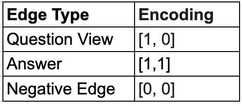
Encoding for Multi Edge Prediction
多边预测编码
Because answering a question requires first viewing it, to score the true probability of an answer, Logit 1 was multiplied by Logit 2. In this way we could capture the relationship between question-view and question-answers in our ranking system. In other words, we used a dependent probability scoring function for answers , calculating P(answer) = P(answer_label) * P(view_label).
因为回答问题需要先查看问题,所以要评分答案的真实概率,就需要将 Logit 1 与 Logit 2 相乘。这样我们就能捕捉到问题查看与问题回答在我们排名系统中的关系。换句话说,我们使用了依赖概率评分函数来评分答案,计算 P(答案) = P(答案标签) * P(查看标签)。
The single stage model had lower computational costs but a different training objective, which we hypothesized would affect the coverage of the trained model, despite using the same data set.
单阶段模型计算成本较低,但训练目标不同,我们假设这会影响训练模型的覆盖率,尽管使用了相同的数据集。
结果
We ran several experiments across GNN model types and with differing features. The first experiment aimed to observe the effect of having a random 3% of the questions labeled with LLM keywords. When experimenting with R-GCNs for link classification, it was observed that cosine similarity for the question embeddings decreased (signifying divergence) even with the small sample size of features. We were eager to see what effect this would have on our GraphSage predictions. In order to do this, we conducted a feature ablation study both with and without the LLM generated features.
我们在 GNN 模型类型和不同特征上进行了多次实验。第一个实验旨在观察随机将 3%的问题用LLM关键词标记的影响。在用 R-GCN 进行链接分类的实验中,观察到问题嵌入的余弦相似度降低(表示发散),即使特征样本量很小。我们急于看到这将对我们的 GraphSage 预测产生什么影响。为了做到这一点,我们进行了带有和不带有LLM生成的特征的特性消除研究。
But first, a short summary description of Precision@K and Recall@K, which are important metrics for our discussion.
但首先,简要介绍一下 Precision@K 和 Recall@K,这两个指标对于我们讨论非常重要。
While accuracy is an important metric in general, it only measures whether predictions are right or wrong. It also requires setting a threshold to determine what counts as a positive prediction. In recommender systems, we are concerned with the quality of our recommendations. Practically speaking, this means we care strongly about the ranking of recommendations and quality of user experience, which can be done by ranking prediction scores. This is where Precision@K and Recall@K come in.
虽然准确率是一个通用的重要指标,但它只衡量预测是正确还是错误。它还需要设置一个阈值来决定什么算作阳性预测。在推荐系统中,我们关注的是推荐的质量。从实际的角度来说,这意味着我们非常关注推荐的排名和用户体验的质量,这可以通过对预测分数进行排名来实现。这就是 Precision@K 和 Recall@K 发挥作用的地方。
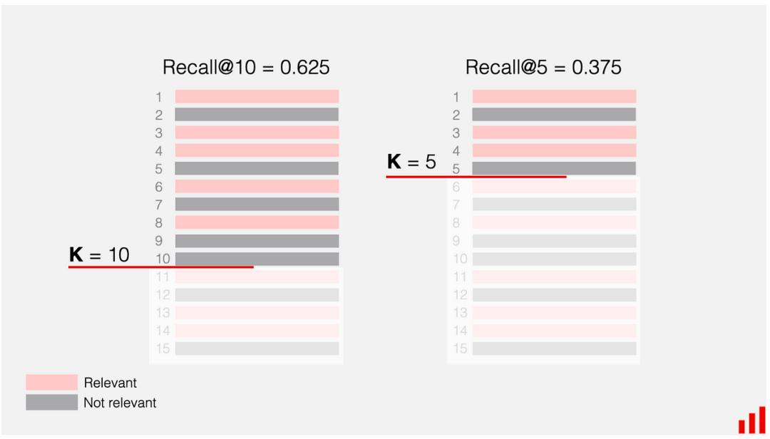
Precision@K measures the proportion of relevant items among the top K recommendations. When looking at our test set, we ask, “Out of K recommendations, how many were actually interacted with by the user?”
Precision@K 衡量的是前 K 个推荐中相关项目的比例。当我们查看测试集时,我们会问:“在 K 个推荐中,有多少是被用户实际互动的?”
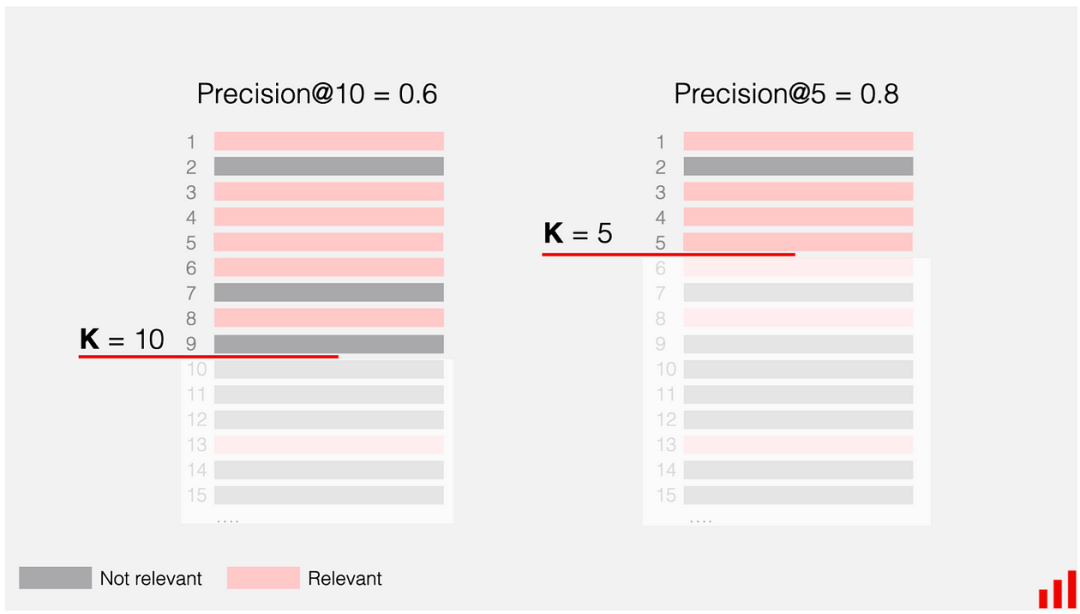
A demonstration of the calculation of Precision@K [2]
Precision@K 的计算演示[2]
Recall@K measures what proportion of all relevant items appear in the top K recommendations. When looking at our test set, we ask, “Out of all of the items the user interacted with, how many did we successfully recommend in the top K?”
Recall@K 衡量了所有相关项目中有多少比例出现在前 K 个推荐中。当我们查看测试集时,我们会问:“在用户互动的所有项目中,我们成功推荐了多少在前 K 个?”
A demonstration of the calculation of Recall@K [2]
Recall@K 的计算演示[2]
To provide context for our metrics, we can consider related work in expert recommendation systems. While not directly comparable, research in the paper, “Expert Finding in Community Question Answering: A Review” considered an excellent precision@5/precision@10 to be ~0.55 [3]. Although their task focused on recommending answers for questions (rather than our approach of recommending questions to answerers), it provides a useful reference point for evaluating recommendation quality in Q&A systems.
为了为我们的指标提供上下文,我们可以考虑专家推荐系统中的相关工作。虽然它们并不直接可比,但论文“社区问答中的专家查找:综述”中认为,一个优秀的 precision@5/precision@10 约为 0.55[3]。尽管他们的任务集中在为问题推荐答案(而不是我们推荐问题给回答者的方法),但它为评估问答系统中的推荐质量提供了一个有用的参考点。
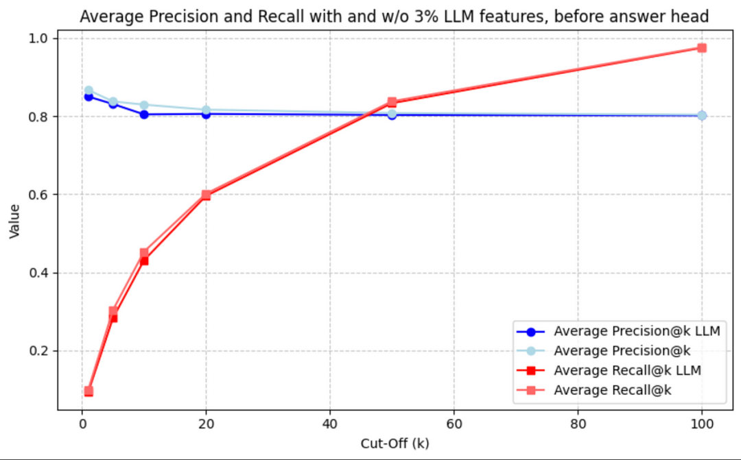
The graph below shows the Precision@K and Recall@K for the view prediction head (before the answer head is trained) both with and without LLM features sprinkled in.
下面的图表显示了在训练答案头之前,带有和不带有LLM特征的情况下,预测头的 Precision@K 和 Recall@K。
Precision@K and Recall@K before answer head is trained
在训练答案头之前,Precision@K 和 Recall@K
Interestingly, the model seems to perform slightly better without the sprinkling of question embeddings, but the performance is largely unaffected. Excluding the LLM features does reduce training times, as would be expected from a reduction of the size of the feature matrices.
有趣的是,模型似乎在没有添加问题嵌入的情况下表现略好,但性能影响不大。排除LLM特征可以减少训练时间,正如从特征矩阵大小的减少所预期的那样。
After the answer head is trained, we see the following:
在训练答案头之后,我们看到了以下结果:
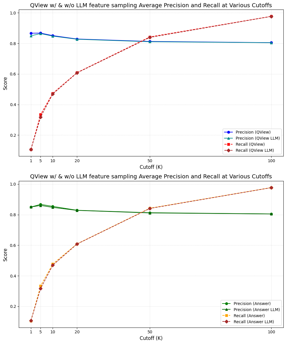
Precision@K and Recall@K for views and answers with and w/o LLM data augmentation — After answer head is trained
在训练答案头之后,对于有和没有LLM数据增强的视图和答案的 Precision@K 和 Recall@K
Again, we can see that the LLM had a very slight negative effect on the performance of the model. This suggests that the LLM data slightly interfered with the learning of the patterns within the data.
再次,我们可以看到LLM对模型性能产生了一点点负面影响。这表明LLM数据略微干扰了数据中模式的学习。
One interesting detail to draw our attention to is the improved performance of the question-view head after training of the answer head. We can see that the precision@K, especially for small K, is improved after training of the answer head. The question-view head was frozen during the training of the answer head so this was initially a surprise.
有一个有趣的细节需要我们注意,那就是在训练答案头之后,问题视图头的性能得到了提升。我们可以看到,在训练答案头之后,特别是对于较小的 K,precision@K 得到了提升。在训练答案头期间,问题视图头被冻结了,这最初是个惊喜。
However, this phenomenon can be attributed to the shared convolutional layers within the GraphSage model. The feature representations in the layers are leveraged for both tasks. Because answer relations are a subset of view relations, answer head training indirectly refines the feature representations that are also used by the question-view head.
然而,这一现象可以归因于 GraphSage 模型中的共享卷积层。这些层中的特征表示被用于两个任务。因为答案关系是视图关系的一个子集,所以答案头的训练间接地细化了也被问题视图头使用的特征表示。
This is analogous to transfer learning, where a model trained on one task can improve performance on related tasks due to the shared knowledge embedded in its feature representations. Learning to predict answers involves understanding user interests and question relevance, which is also crucial for predicting question-views.
这与迁移学习类似,迁移学习是指一个在某个任务上训练好的模型可以通过其特征表示中嵌入的共享知识来提高相关任务的表现。预测答案的学习涉及理解用户兴趣和问题相关性,这对于预测问题浏览量也是至关重要的。
GraphSage Multi-dimensional Edge Label Model
GraphSage 多维边标签模型
To demonstrate the utility of the transfer learning like approach of staged task learning, we also experimented with a different GraphSage model architecture, which attempted to encode both question-view and question-answer prediction tasks in a single model with two output logits per edge. To this end, we conducted an architecture ablation study to see the effect of one stage vs two stage learning of question-views and question-answer relations.
为了展示类似迁移学习的分阶段任务学习方法的实用性,我们还尝试了一种不同的 GraphSage 模型架构,该架构试图在一个模型中编码问题浏览和问题回答预测任务,每个边有两个输出对数。为此,我们进行了一次架构消融研究,以观察单阶段学习与双阶段学习在问题浏览和问题回答关系上的影响。
Prior to this, we also conducted a model component ablation study to see the optimal layer size for our GraphSage model, centered around the one stage model. In our tests of the effect of layer counts, we observed training loss and validation loss dropping pretty similarly despite the differences. Therefore, for further testing, we used a 3 layer network. We additionally did not use LLM data for comparison to the two stage GraphSage prediction training results.
在此之前,我们还进行了一项模型组件消融研究,以确定 GraphSage 模型的最佳层大小,主要集中在单阶段模型上。在我们的层计数效应测试中,观察到训练损失和验证损失下降相当相似,尽管存在差异。因此,为了进一步测试,我们使用了 3 层网络。此外,我们没有使用LLM数据与两阶段 GraphSage 预测训练结果进行比较。
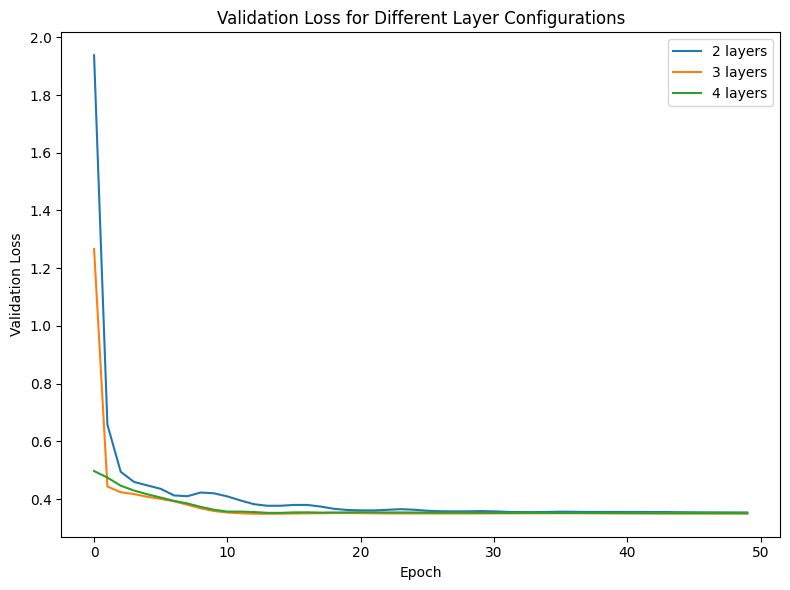
Here we can see the validation loss curves for various layer counts
这里我们可以看到各种层计数的验证损失曲线。
This experimentation led to quite an interesting result.
这项实验产生了一个相当有趣的结果。
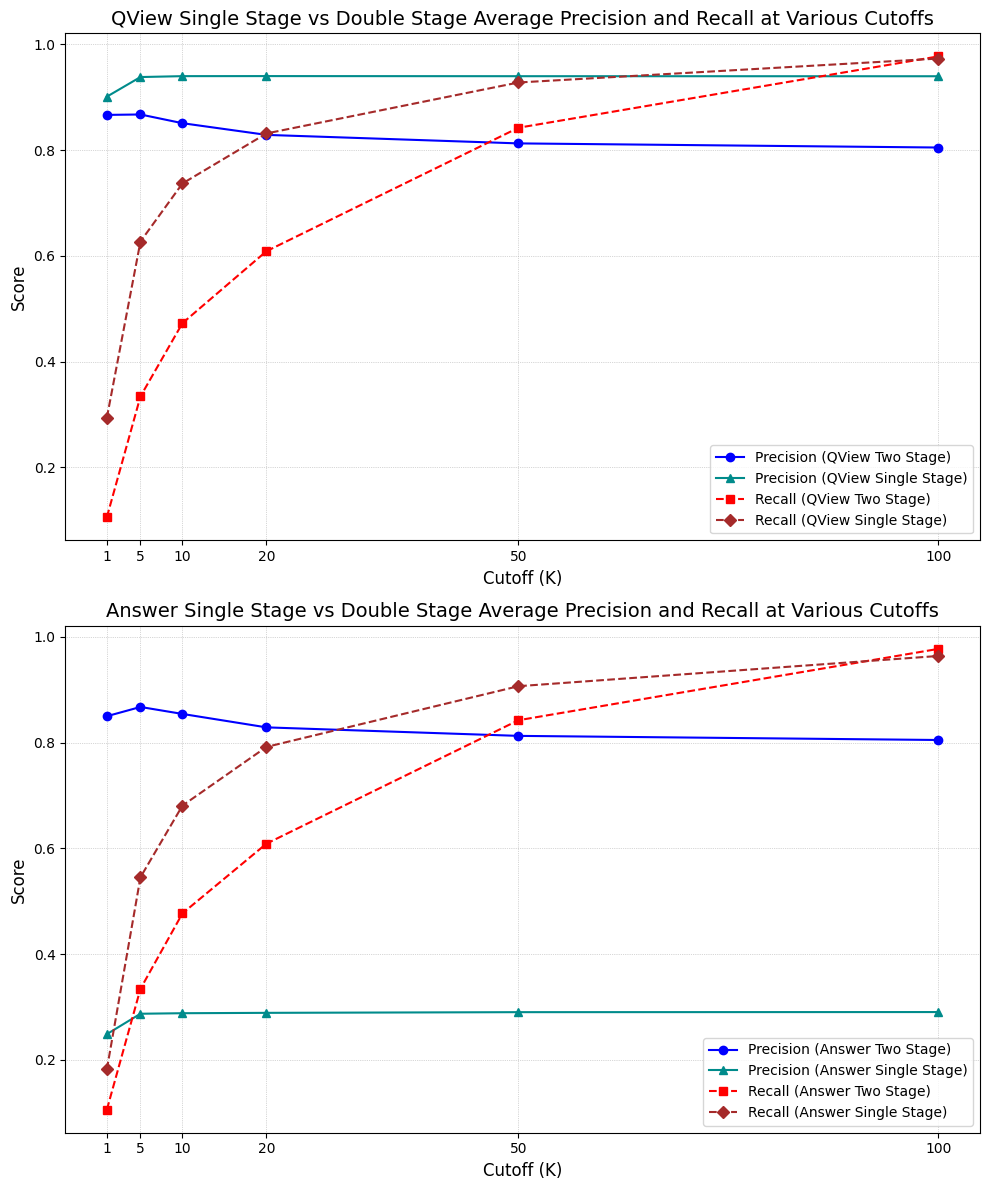
Comparison of Precision@K and Recall@K between single stage and two stage training for question views and question answers.
对问答视图和问答的 Precision@K 和 Recall@K 在单阶段和两阶段训练之间的比较。
The single stage GNN (training both labels simultaneously) outperformed the two stage GNN (training the prediction heads one at a time) in question-view precision and recall (although two stage matched recall for high K). However, single stage greatly suffered in answer precision. While single stage also outperformed two stage in recall for smaller K, for higher K, the two stage GNN outperformed the single stage.
单阶段 GNN(同时训练两个标签)在问题视图的精确度和召回率方面优于两阶段 GNN(逐个训练预测头),尽管两阶段在 K 值较高时召回率相当。然而,单阶段在答案精确度方面明显下降。虽然单阶段在 K 值较小时召回率优于两阶段,但对于 K 值较高的情况,两阶段 GNN 在召回率方面优于单阶段。
We theorize this occurred because training for both labels at once, in a single stage, forced the GNN to balance competing objectives, focusing on more easily distinguishable patterns that maximize precision but struggle with recall. It is also likely that the presence of the answer signal amplified the question view signal. In domains where precision@K for the superset is prioritized, it makes sense to train in a single stage. If there isn’t much overlap between labels, it may also make sense to simply use a single stage model.
我们认为这是由于单阶段同时训练两个标签,迫使 GNN 平衡竞争目标,关注于更容易区分的模式,以最大化精确度但召回率方面存在困难。答案信号的存在也可能放大了问题视图信号。在优先考虑子集的 precision@K 的领域,单阶段训练是有意义的。如果标签之间没有太多重叠,也可能简单地使用单阶段模型。
In the medical domain, where coverage in the form of recall is just as important as precision, we believe it makes sense to adopt robustness of the two stage model. As a drawback, the two stage model does require more computational resources. However, answers are a very valuable part of the medical discussion. The medical community would greatly benefit from more answers to their questions — and by predicting the questions that a user can answer, we can greatly aid the healthcare system.
在医学领域,召回率与精确率一样重要,我们认为采用两阶段模型的鲁棒性是有意义的。然而,两阶段模型确实需要更多的计算资源。然而,答案在医学讨论中是非常宝贵的。医学界将从更多的问题答案中受益——通过预测用户可以回答的问题,我们可以极大地帮助医疗保健系统。
R-GCN 模型
We also investigated the utility of R-GCNs for this task. While not suited to inductively reason on the data, we would be able to utilize a more complex graph structure to make recommendations. For the R-GCN, we added publication nodes and edges between publications, doctors, and questions. We also added edge-weights to learn edge specific mappings between nodes and triplet loss using cosine similarity that specifically optimizes for view and answer interactions. Because the R-GCN had many relation types, it was much more computationally expensive and necessitated the use of data loaders and batching to compute on the Google Colab available GPUs. The training times were long and did not yield promising results for recall@K and precision@K, even after many epochs had elapsed. While losses would drop, node embeddings did not diverge sufficiently from those of the same type. Adding LLM generated question features to a random 3% of questions did decrease cosine similarity, but not sufficiently to significantly improve recommendation quality. Below is a sample snapshot of the unpromising validation metrics.
我们也研究了 R-GCNs 在此任务中的效用。虽然不适合对数据进行归纳推理,但我们能够利用更复杂的图结构来做出推荐。对于 R-GCN,我们添加了出版物节点以及出版物、医生和问题之间的边。我们还添加了边权重,通过余弦相似度学习节点和三元组损失之间的特定映射,以优化视图和答案交互。由于 R-GCN 有许多关系类型,它计算成本更高,需要使用数据加载器和批处理来在 Google Colab 可用的 GPU 上计算。训练时间很长,即使经过许多个 epoch,也没有在 recall@K 和 precision@K 上产生有希望的结果。虽然损失会下降,但节点嵌入并没有足够地从同一类型的嵌入中发散出来。将LLM生成的问答特征添加到随机 3%的问题中确实降低了余弦相似度,但不足以显著提高推荐质量。以下是未达到预期效果的验证指标样本快照。
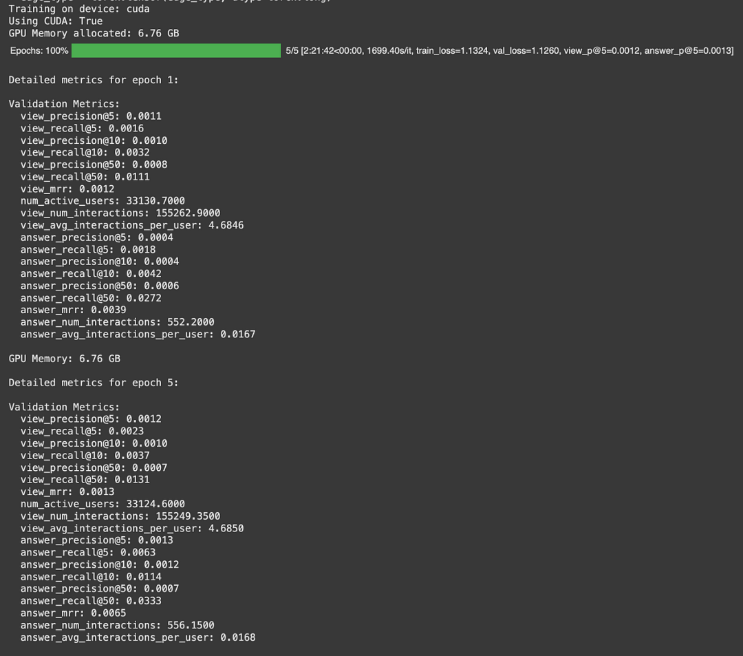
Marginal improvement in R-GCN metrics after 5 epochs and ~2.5 hours of training time
经过 5 个 epoch 和约 2.5 小时的训练时间后,R-GCN 指标有所提升
结论
In this project, we explored a number of different GNN model architectures to improve recommendations of questions to doctors. The most effective GNN was a GraphSage based model that leveraged multiple prediction heads to gain transfer learning like improvements in model representation, leading to improvements in recommendations as captured by improved Recall@K and Precision@K.
在这个项目中,我们探索了多种不同的 GNN 模型架构,以改进向医生推荐问题的推荐。最有效的 GNN 是一个基于 GraphSage 的模型,该模型利用多个预测头实现了类似迁移学习的改进,从而提高了模型表示,进而提高了推荐质量,这体现在改进的 Recall@K 和 Precision@K 上。
Starting with question-view edge predictions as a foundation, we experimented with training prediction heads for additional question-doctor relation types. By leveraging the strengths of the question-view predictions, we started the training of the prediction of answer edges at a high level. This training, in turn, improved the overall performance of the question-view predictions.
从问题视图边预测作为基础开始,我们尝试训练预测头以预测额外的问答关系类型。通过利用问题视图预测的优势,我们开始以较高水平训练答案边的预测。这种训练反过来又提高了问题视图预测的整体性能。
This double stage model outperformed the single stage model for the purposes of our medical Q&A domain, but it did not outperform the single stage model in all metrics, which excelled in precision@K, especially for smaller numbers of k and for the label superset.
这种双阶段模型在我们的医疗问答领域优于单阶段模型,但在所有指标上并未优于单阶段模型,特别是在精度@K 方面,特别是在 k 值较小和标签全集的情况下。
Because our GNN is inductive, we will be able to use it to make better recommendations for both new physician users and old physician users who may not have taken any actions on the site yet. We also look forward to continuing to experiment with LLM generated features and graph structures to continue to improve recommendations.
因为我们的 GNN 是归纳的,所以我们将能够用它为新医生用户和可能尚未在网站上采取任何行动的旧医生用户提供更好的推荐。我们也期待继续实验LLM生成的特征和图结构,以继续改进推荐。
We’re very excited to use these techniques to improve physician access to relevant information for their practices, hopefully improving the health of people across the world via this conduit to expert level medical advice. Hope you’re excited as well and that you enjoyed this read!
我们非常兴奋地使用这些技术来改善医生获取与其实践相关的信息,希望通过这条通往专家级医疗建议的途径改善世界各地人们的健康。希望您也感到兴奋,并且喜欢这次阅读!
参考文献
[1] themednet.org
[2] https://www.evidentlyai.com/ranking-metrics/precision-recall-at-k
[3] Yuan S., et. al. Expert Finding in Community Question Answering: A Review. https://arxiv.org/pdf/1804.07958


内容中包含的图片若涉及版权问题,请及时与我们联系删除

评论
沙发等你来抢