
Stanford CS224W: Machine Learning with Graphs
By Josfran as part of the Stanford CS 224W Final Project
https://github.com/tnguyen2002/graphsketball
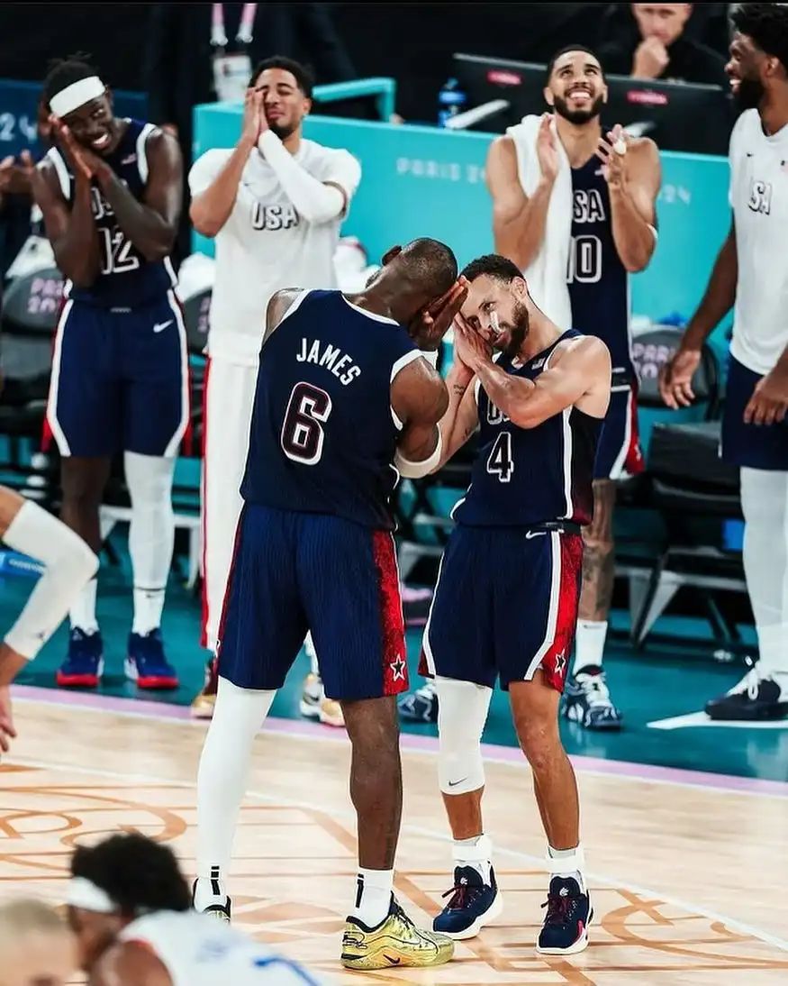
Curry and his future teammates
库里和他未来的队友
How are the Warriors going to do this year given how tough the Western Conference is? Which star players should the Warriors try to trade for to bolster their chances of success and making the playoffs in one of Curry’s last years? If cap restrictions weren’t an issue, which superstar would capitalize off of Curry’s spacing? Giannis? Jokic?
考虑到西部联盟的艰难程度,勇士队今年的表现如何?勇士队应该尝试交易哪些明星球员,以增加他们在库里的最后几年取得成功和进入季后赛的机会?如果上限限制不是一个问题,哪位超级巨星会利用库里的间距呢?扬尼斯?约基奇?
These are all questions that we and many other Warriors fans have wondered both this season and many seasons before. But I’ve never been able to answer these questions, until now. Enter Graphsketball: a project designed to leverage Graph Neural Networks (GNNs) to uncover insights into player relationships, team dynamics, and trade optimization.
这些都是我们和许多其他勇士球迷在本赛季和之前许多赛季都想知道的问题。但直到现在,我一直无法回答这些问题。进入 Graphsketball:一个旨在利用图神经网络 (GNN) 来揭示玩家关系、团队动态和交易优化的洞察的项目。
To start, we tried to explore player chemistry and which players pair well together. To do so, we extracted a dataset of 20 seasons worth of per-player per-season advanced stats. We thought of every player as a node, their stats as node features, and we connected two players if they’ve ever played together. We set the edge weight as the average combined box plus minus of the two players across all seasons they played together. Box plus minus (BPM) is an advanced stat that encapsulates various variables like rebounds, points, steals, etc while the player is on the floor versus off, so overall it measures their impact when on the floor. Our thinking was that if a player’s BPM was higher when on the same team as another player, then those two players had chemistry, so this metric would be a proxy measure of player chemistry.
首先,我们尝试探索玩家的化学反应以及哪些玩家可以很好地配对 。为此,我们提取了一个包含 20 个赛季每个赛季每个球员的高级统计数据的数据集。我们将每个玩家都视为一个节点,他们的统计数据被视为节点特征,如果他们曾经一起玩过,我们会将两个玩家连接起来。我们将边权重设置为两名球员在他们一起打的所有赛季中的平均总和箱加减。箱加负值 (BPM) 是一种高级统计数据,它封装了球员在场上与场下时的各种变量,如篮板、得分、抢断等,因此总体而言,它衡量了他们在场上时的影响。我们的想法是,如果一名球员与另一名球员在同一支球队时 BPM 更高,那么这两名球员就有化学反应,所以这个指标将是球员化学反应的代理衡量标准。
So, we set up our graph and edge weights, and trained a Graph Convolutional Network (GCN) to learn node embeddings, such that when we took the dot product of two nodes’ embeddings, it would give the right edge weight. This edge weight prediction task was a regression task, which we used the Mean Squared Error (MSE) loss/evaluation function for.
因此,我们设置了图形和边缘权重,并训练了一个图形卷积网络 (GCN) 来学习节点嵌入,这样当我们取两个节点嵌入的点积时,它会给出正确的边缘权重。这个边缘权重预测任务是一个回归任务,我们使用了均方误差 (MSE) 损失/评估函数。
Validation MSE for Edge Weight Regression
用于 Edge 权重回归的验证 MSE
We found that our model had very low MSE very quickly, before getting quite unstable. To test how good our performance was, we then constructed some baseline models to compare against. We first trained a logistic regression model, which ultimately got a training MSE of 47.4937,
我们发现我们的模型很快就具有非常低的 MSE,然后变得非常不稳定。为了测试我们的性能有多好,我们构建了一些基线模型进行比较。我们首先训练了一个 logistic 回归模型 ,最终得到的训练 MSE 为 47.4937,
a validation MSE of 47.4937, and a test MSE of 48.0408. Our next baseline was a random forest model, which got a much better training MSE of 0.9989, a validation MSE of 0.9989, and a test MSE of 3.0995.
验证 MSE 为 47.4937,测试 MSE 为 48.0408。我们的下一个基线是一个随机森林模型,它的训练 MSE 要好得多,为 0.9989,验证 MSE 为 0.9989,测试 MSE 为 3.0995。
Our random forest model was nearly as good as our model, and our model was suspiciously good, so we dug into the weights a bit and realized that since BPM was one of our node features, the model was basically just learning how to take an average of the two nodes. This was not super meaningful, so we decided to switch to a different approach that was more meaningful.
我们的随机森林模型几乎和我们的模型一样好,而且我们的模型好得可疑,所以我们稍微深入研究了权重,并意识到由于 BPM 是我们的节点特征之一,因此该模型基本上只是在学习如何取两个节点的平均值。这并不是特别有意义,所以我们决定改用更有意义的不同方法。
Instead of constructing our own proxy measure and trying to parse player-to-player interactions out of our dataset, we started to think about what our dataset was actually telling us. We had player data over 20 years, but it would be really hard to identify how the player was doing in a vacuum or how two players were doing irrespective of the players around them, because player performance is so dependent on the team they’re on. What we did realize though was that our graph has team data, so our data was well suited for team-level prediction tasks instead of edge-level prediction.
我们没有构建自己的代理度量并尝试从数据集中解析玩家与玩家的交互,而是开始思考数据集实际上告诉我们什么。我们拥有 20 多年的球员数据,但无论周围的球员是谁,都很难确定球员在真空中的表现如何,或者无论他们周围的球员是谁,都很难确定他们是如何表现的,因为球员的表现非常取决于他们所在的球队。但我们确实意识到,我们的图表包含团队数据,因此我们的数据非常适合团队级别的预测任务,而不是边缘级别的预测。
Because of this, we turned to a new task: predicting team wins. We chose this prediction task because not only is it well suited to our data, it also let’s see how players play together, in a clever way that we will discuss in a bit.
因此,我们转向了一项新任务: 预测团队获胜 。我们选择这个预测任务,不仅因为它非常适合我们的数据,而且还让我们看到玩家如何一起玩,以一种聪明的方式,我们稍后会讨论。
To predict team wins, we got an accompanying dataset of the NBA standings for the last 20 years, including every team’s wins and losses. From this, we designed a new model, shown below.
为了预测球队的胜场数,我们得到了过去 20 年 NBA 排名的随附数据集,包括每支球队的胜负。由此,我们设计了一个新模型,如下所示。
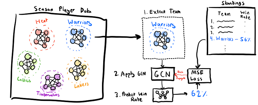
One-Tier Model 单层模型
The goal of our initial model was simple: train a GNN to take in a subgraph for a specific team, and predict its wins and losses. Instead of our original graph where we had every player from all seasons in one graph, we have one graph per season, and we further extract out the subgraph for each team. We end up with just the 2022 Warriors graph for example, and we get that they had 53 wins. We then run a GCN on the subgraph, run it through a linear prediction head, and get a predicted win count, for example 60. We then take the mean squared error loss between the prediction and true wins, so (60–53)² = 7² = 49, and do the same for every team across every year. Once we have the total loss, we back-propagate it into the GCN model to update the weights and make better predictions next time.
我们初始模型的目标很简单:训练一个 GNN 来获取特定球队的子图,并预测其胜负。我们原来的图表中将所有赛季的每位球员都放在一个图表中,而不是我们每个赛季都有一个图表,然后我们进一步提取出每支球队的子图表。例如,我们最终只得到了 2022 年勇士队的图表,我们得到他们有 53 场胜利。然后,我们在子图上运行 GCN,通过线性预测头运行它,并获得预测的获胜计数,例如 60。然后,我们取预测和真实胜场之间的均方误差损失,即 (60–53)² = 7² = 49,并对每年的每支球队进行相同的作。一旦我们有了总损失,我们就会将其反向传播到 GCN 模型中,以更新权重并在下次做出更好的预测。
This initial baseline worked well, producing the following predictions for this upcoming season:
这个初始基线运行良好,为即将到来的赛季产生了以下预测:
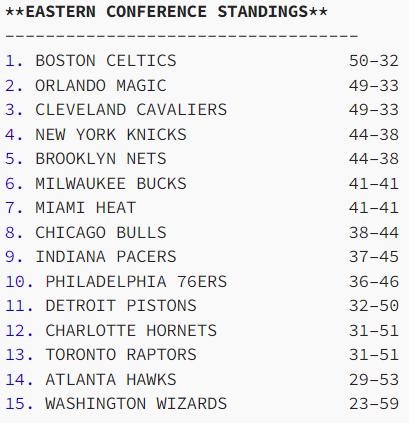
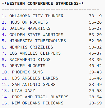
For anybody who is following the NBA this season, this is surprisingly accurate. What’s even more surprising is that these predictions only take into accout a single team’s player stats. It’s basically looking at the Warriors, saying “Oh, they have lots of good shooters but not great rebounding” and then producing predicted wins. It actually doesn’t take into account the other teams, at least when predicting. Technically the information is somewhat accounted for given that the model sees all teams over the course of training, but it doesn’t know how the Warriors compare to other teams in a certain season. So, despite how well this model did, we decided to try making yet another model to handle this model’s limitations. This leads us to our next model, shown below:
对于任何关注本赛季 NBA 的人来说,这都是出奇的准确。更令人惊讶的是,这些预测只考虑了单个球队的球员统计数据。这基本上是看着勇士队,说“哦,他们有很多优秀的射手,但篮板球不是很好”,然后产生预测的胜利。它实际上没有考虑到其他球队 ,至少在预测时是这样。从技术上讲,该模型在一定程度上考虑了这些信息,因为该模型在训练过程中看到了所有球队,但它不知道勇士队在某个赛季与其他球队的比较情况。因此,尽管这个模型做得非常好,我们还是决定尝试制作另一个模型来处理这个模型的局限性。这导致我们进入下一个模型,如下所示:
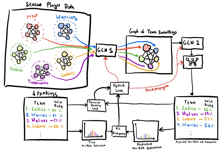
Two-Tier Model 两层模型
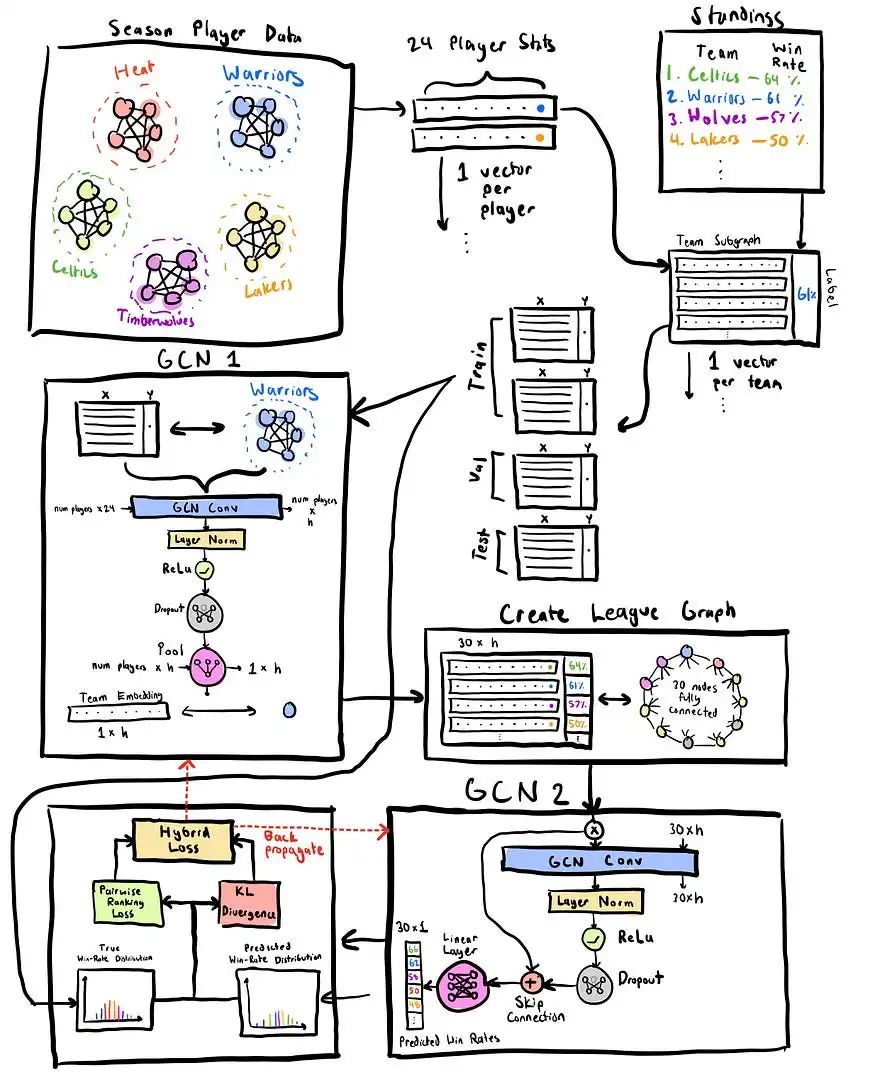
This model starts out slightly differently, as it keeps a season’s graph intact rather than splitting it up by team. It then runs each team through the same GCN architecture from before, but without the prediction head. What this means is that it produces an embedding vector for each team, or a team embedding, rather than a wins prediction. This team embedding ideally captures how well the team is doing, and we can then compare it against the embeddings for other teams in the league. To do so, we then construct a team graph, where there’s a node for each team with its feature vector being its corresponding team embedding, and then all nodes are connected to each other. Finally, we run a second GCN on top of this graph, and get win predictions for every node/team in the graph. These win predictions are then compared against the whole standings for that season, and the loss is propagated back through.
这个模型的开始略有不同,因为它保持赛季图表不变,而不是按球队划分。然后,它通过与之前相同的 GCN 架构运行每个团队,但没有预测头。这意味着它为每个团队生成一个嵌入向量 ,或者一个团队嵌入向量,而不是一个获胜预测。这个球队嵌入理想地捕捉了球队的表现,然后我们可以将其与联盟中其他球队的嵌入进行比较。为此,我们构建了一个团队图 ,其中每个团队都有一个节点,其特征向量是其相应的团队嵌入,然后所有节点都相互连接。最后,我们在此图表上运行第二个 GCN,并获得图表中每个节点/团队的获胜预测。然后将这些获胜预测与该赛季的整个排名进行比较,并将损失传播回去。
Here we had to make a key design decision. Although MSE worked well for our simpler model, the two-tiered model was really tricky to train. What we found is that when predicting a bunch of team wins, it would predict really close to 42, since that’s the average wins for all teams in a certain season. It would get good performance but end up stuck in a local minimum, but not the global minimum. So, we had to come up with a new loss function to encourage it to get out of this hole.
在这里,我们必须做出一个关键的设计决策。尽管 MSE 适用于我们更简单的模型,但两层模型确实很难训练。我们发现,当预测一堆球队的胜利时,它会预测非常接近 42 场,因为这是某个赛季所有球队的平均胜利。它会获得良好的性能,但最终会卡在局部最小值 ,而不是全局最小值 。因此,我们必须想出一个新的损失函数来鼓励它走出这个坑。
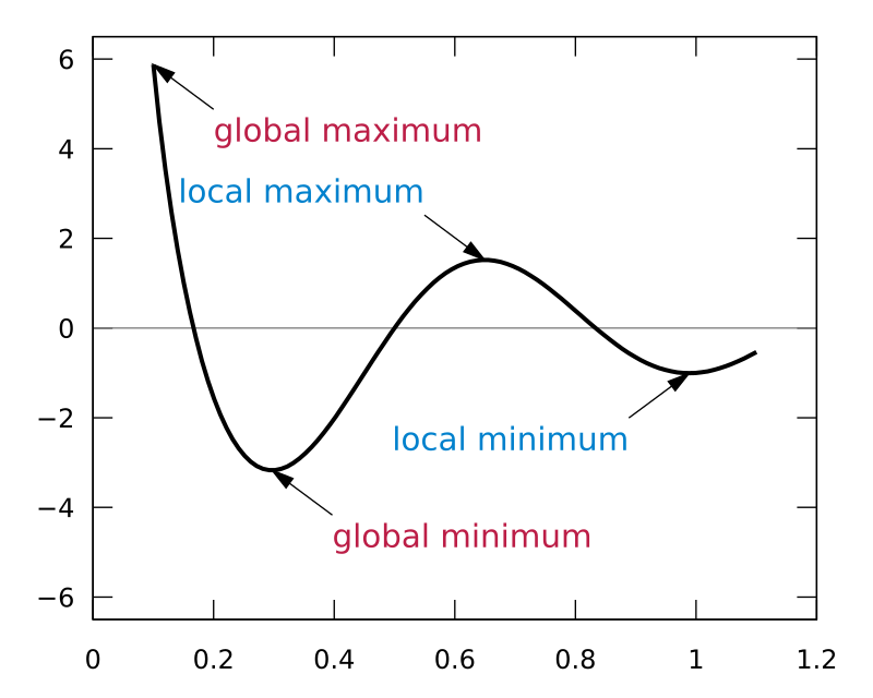
Our model was initially stuck in a local minimum with MSE, so we had to design a new loss function to help it find the global minimum
我们的模型最初卡在 MSE 的局部最小值中,因此我们不得不设计一个新的损失函数来帮助它找到全局最小值
After a few iterations we settled on a custom hybrid loss function. Our custom loss function came from a few observations. One was that the most important thing was the ordering of teams. It would be okay if the teams’ wins were slightly off as long as their overall ordering was wrong. So, we looked into loss functions that penalize incorrect orderings of pairs of predictions, and came across the Pairwise Ranking Loss function, which does exactly that.
经过几次迭代,我们确定了一个自定义的 hybrid loss 函数 。我们的自定义损失函数来自一些观察。一个是最重要的事情是团队的顺序。如果球队的胜场数略有偏差,只要他们的整体顺序是错误的,那也没关系。因此,我们研究了对预测对的错误排序进行惩罚的损失函数,并发现了 Pairwise Ranking Loss 函数,它正是这样做的。
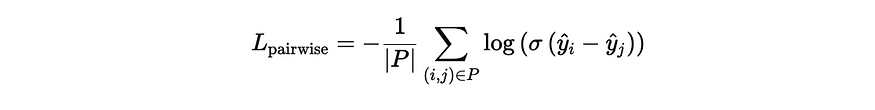
Pairwise Ranking Loss 成对排名损失
However, when we then trained our model with our pairwise ranking loss, it had the right ordering, but half the teams would be roughly 82–0, and the other half would be roughly 0–82. So, it got the right ordering, but at the complete expense of having a reasonable distribution. Basically, the pairwise ranking loss was completely ignoring the value of the wins and only looking at relative ordering, so we needed to augment this loss function with something that would enforce a reasonable distribution. To do this, we guessed that the wins would be roughly a normal distribution centered around a 0.5 win percentage (winning half the time), but we weren’t exactly sure what the variance would be, so we created a program that fit the past 20 years of NBA win distributions to a normal distribution and found the following:
然而,当我们用成对排名损失训练我们的模型时,它的顺序是正确的,但一半的球队大约是 82-0,另一半大约是 0-82。因此,它得到了正确的排序,但完全以合理的分配为代价。基本上,成对排名损失完全忽略了胜利的值,只关注相对排序,因此我们需要用一些能够强制执行合理分配的东西来增强这个损失函数。为此,我们猜测胜场大致是一个以 0.5 胜率为中心的正态分布(胜率占一半),但我们并不完全确定方差会是多少,因此我们创建了一个程序,将过去 20 年的 NBA 胜场分布拟合到正态分布,并发现以下内容:
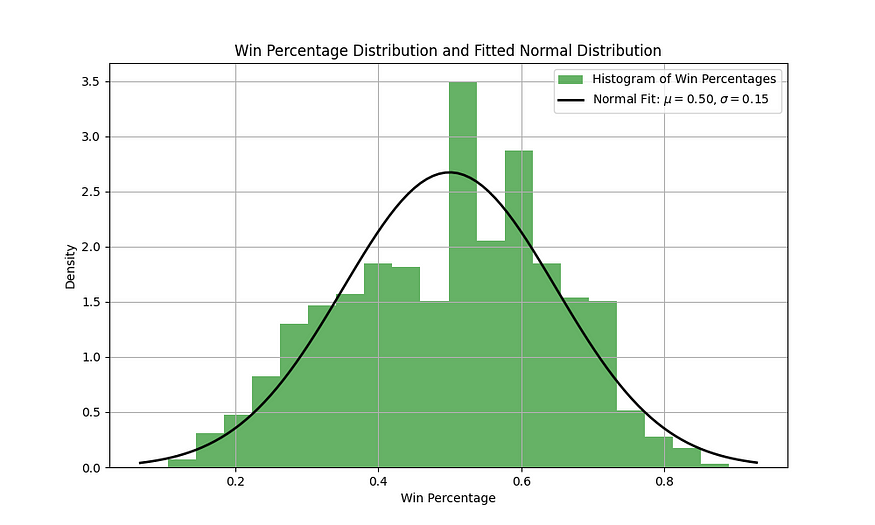
Like we thought, wins follow a roughly normal distribution centered around a 50% win percentage, with a standard deviation of 15%. Using this, we added a term to the loss function that enforces this distribution, and used KL-Divergence to penalize the model for outputting values far away from this distribution, with the equation for KL-Divergence shown below.
正如我们所想的,胜率大致呈正态分布,胜率为 50%,标准差为 15%。利用这一点,我们在损失函数中添加了一个强制执行此分布的项,并使用 KL-Divergence 来惩罚模型输出远离此分布的值,KL-Divergence 的方程如下所示。
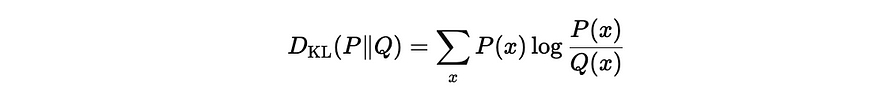
KL Divergence Formula, used for forcing a normal distribution of wins
KL Divergence Formula(KL 背离公式),用于强制胜场呈正态分布
We then designed our final loss function to be the following:
然后,我们将最终的损失函数设计为:
Our final loss function 我们最终的损失函数
In our case, we found that weighting the pairwise loss as 90% and the distribution constraint loss as 10% worked well. With this, we then trained the model, with details shown below:
在我们的例子中,我们发现将成对损失加权为 90%,将分布约束损失加权为 10% 效果很好。然后,我们训练了模型,详细信息如下所示:
Full details for our final model
我们最终模型的完整详细信息
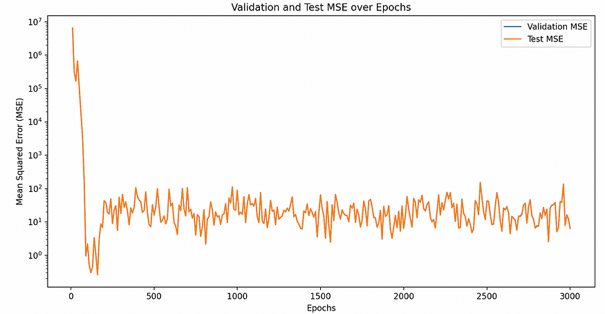
Training was still tricky, requiring us to use learning rate schedulers and regularization to make sure that the model didn’t overfit or underfit. Our final training plots are shown below:
训练仍然很棘手,需要我们使用学习率调度器和正则化来确保模型不会过度拟合或欠拟合。我们最终的训练图如下所示:
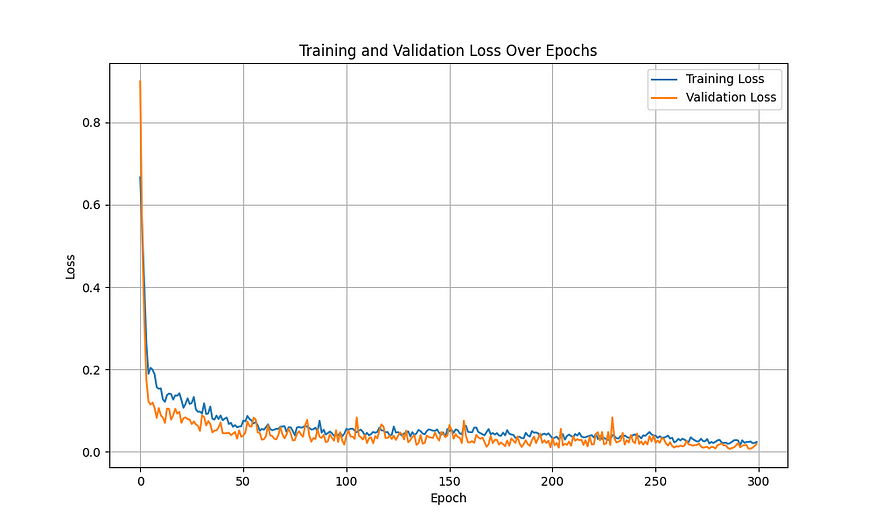
Final Training Plots for Final Model
最终模型的最终训练图
With this, our model was done, and it was time to test it out. First, its predictions for the upcoming season:
这样,我们的模型就完成了,是时候对其进行测试了。首先,它对即将到来的赛季的预测:
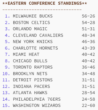
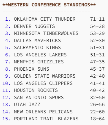
These predictions were also really good, so we then wrote a program to compare the two. The results were mixed:
这些预测也非常好,因此我们随后编写了一个程序来比较两者。结果喜忧参半:
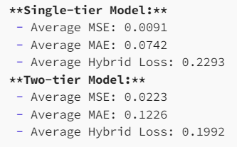
What’s interesting is that the single-tier model, although simpler, was able to achieve a lower MSE than the more advanced model. However, the hybrid loss was better for the two-tiered model. This makes sense given that these were the loss functions that each model trained on, but it’s still impressive that the model that doesn’t take into account the other teams in the league would be able to outperform one with that context.
有趣的是,单层模型虽然更简单,但能够实现比更高级的模型更低的 MSE。然而,两层模型的混合损失更好。这是有道理的,因为这些是每个模型训练的损失函数,但令人印象深刻的是,不考虑联盟中其他球队的模型能够在该背景下胜过一支球队。
The beauty of this model is that although its training is slow, its prediction is actually really quick, so we could now finally answer our starting questions: which superstar would best accompany Curry, and which stars should the Warriors trade for?
这个模型的美妙之处在于,虽然它的训练很慢,但它的预测实际上真的很快,所以我们现在终于可以回答我们的起始问题了: 哪位超级巨星最适合陪伴库里 ,勇士应该交易哪些球星 ?
For the first question, we created a program that tried moving every player in the whole league from their existing team to the Warriors, and then running predictions. We got the following results:
对于第一个问题,我们创建了一个程序,尝试将整个联盟中的每个球员从他们现有的球队转移到勇士队,然后运行预测。我们得到了以下结果:
1. Shai Gilgeous-Alexander (from OKLAHOMA CITY THUNDER): +0.2983 improvement in predicted win%
2. Nikola Jokić (from DENVER NUGGETS): +0.1677 improvement in predicted win%
3. Giannis Antetokounmpo (from MILWAUKEE BUCKS): +0.1664 improvement in predicted win%
4. Kyrie Irving (from DALLAS MAVERICKS): +0.1591 improvement in predicted win%
5. Anthony Davis (from LOS ANGELES LAKERS): +0.1513 improvement in predicted win%
6. Jayson Tatum (from BOSTON CELTICS): +0.1433 improvement in predicted win%
7. Franz Wagner (from ORLANDO MAGIC): +0.1352 improvement in predicted win%
8. Anthony Edwards (from MINNESOTA TIMBERWOLVES): +0.1331 improvement in predicted win%
9. De'Aaron Fox (from SACRAMENTO KINGS): +0.1254 improvement in predicted win%
10. Donovan Mitchell (from CLEVELAND CAVALIERS): +0.1090 improvement in predicted win%
However, these additions are unfortunately unrealistic, because they assume that we get the player without giving anything in return. That leads us to our final application, which is finding all win-win trades. Since our prediction is so fast, we can once again exhaustively search all options: for every Warriors player, try trading with every other player in the league, then find all trades that are mutually beneficial (but benefitting the Warriors more than the other team), and then rank them by how beneficial they are. The results were quite surprising:
然而,不幸的是,这些添加是不现实的,因为它们假设我们得到了玩家而不给予任何回报。这就引出了我们的最后一个应用程序,即找到所有双赢的交易 。由于我们的预测如此之快,我们可以再次详尽地搜索所有选项:对于每个勇士队球员,尝试与联盟中的其他所有球员进行交易,然后找到所有互惠互利的交易(但对勇士队的益处大于其他球队),然后根据它们的收益程度对它们进行排名。结果相当令人惊讶:
1. Swap Stephen Curry (GSW) with Jalen Williams (OKLAHOMA CITY THUNDER)
   Warriors improvement: 0.1040
   OKLAHOMA CITY THUNDER improvement: 0.0022
2. Swap Stephen Curry (GSW) with Damian Lillard (MILWAUKEE BUCKS)
   Warriors improvement: 0.0847
   MILWAUKEE BUCKS improvement: 0.0153
3. Swap Stephen Curry (GSW) with Karl-Anthony Towns (NEW YORK KNICKS)
   Warriors improvement: 0.0829
   NEW YORK KNICKS improvement: 0.0210
4. Swap Jonathan Kuminga (GSW) with Jalen Williams (OKLAHOMA CITY THUNDER)
   Warriors improvement: 0.0770
   OKLAHOMA CITY THUNDER improvement: 0.0017
5. Swap Brandin Podziemski (GSW) with Jalen Williams (OKLAHOMA CITY THUNDER)
   Warriors improvement: 0.0758
   OKLAHOMA CITY THUNDER improvement: 0.0298
6. Swap Kevon Looney (GSW) with Jalen Williams (OKLAHOMA CITY THUNDER)
   Warriors improvement: 0.0732
   OKLAHOMA CITY THUNDER improvement: 0.0355
7. Swap Trayce Jackson-Davis (GSW) with Jalen Williams (OKLAHOMA CITY THUNDER)
   Warriors improvement: 0.0728
   OKLAHOMA CITY THUNDER improvement: 0.0356
8. Swap Draymond Green (GSW) with Jalen Williams (OKLAHOMA CITY THUNDER)
   Warriors improvement: 0.0723
   OKLAHOMA CITY THUNDER improvement: 0.0344
9. Swap Kyle Anderson (GSW) with Jalen Williams (OKLAHOMA CITY THUNDER)
   Warriors improvement: 0.0721
   OKLAHOMA CITY THUNDER improvement: 0.0374
10. Swap De'Anthony Melton (GSW) with Jalen Williams (OKLAHOMA CITY THUNDER)
   Warriors improvement: 0.0717
   OKLAHOMA CITY THUNDER improvement: 0.0368
Shockingly, the model has decided to go against my goal of finding a superstar to pair with Curry, and has instead decided to do the worst thing possible: trade Curry. However, it’s suggestions are surprisingly good outside of that. The model seems to have a strong sense of player roles, despite that not being explicitly designed into the model. We gave the model player stats and player position, and it somehow knows from that Curry and Dame are similar, as are Podziemski and Jalen Williams. It knows what the Warriors need, and what other teams have to offer. Also, we didn’t include it here since it would take up too much space, but each of these predictions comes with a full set of standings, so not only can you see the impact of Kuminga and Jalen Williams on OKC and the Warriors, but you can also see how that affects other teams in the league and changes power dynamics.
令人震惊的是,这位模特决定违背我寻找超级巨星与 Curry 配对的目标,而是决定做最糟糕的事情: 交易 Curry。然而,它的建议出奇地好。该模型似乎具有很强的玩家角色意识,尽管它没有明确设计到模型中。我们给出了模型球员的统计数据和球员位置,它以某种方式知道库里和达姆很相似,波齐姆斯基和杰伦威廉姆斯也是如此。它知道勇士队需要什么,也知道其他球队必须提供什么。此外,我们没有将其包含在这里,因为它会占用太多空间,但这些预测中的每一个都带有一整套排名,因此您不仅可以看到 Kuminga 和 Jalen Williams 对 OKC 和勇士队的影响,还可以看到它如何影响联盟中的其他球队并改变权力动态。
Overall, this project was mainly for fun, but it does show the potential for Graph ML to be used in sports analytics. An easy next step which we almost included in this project is making a lightweight web app that lets you move players around from team to team and see how standings change, alongside recommended trades. This would let teams see how to leverage their assets and make win-win trade package offers to other teams to slowly improve their standing.
总的来说,这个项目主要是为了好玩,但它确实显示了 Graph ML 在体育分析中的潜力。我们几乎包含在该项目中的一个简单的下一步是制作一个轻量级的 Web 应用程序,让玩家从一个团队移动到另一个团队,并查看排名如何变化,以及推荐的交易。这将使团队了解如何利用他们的资产并向其他团队提供双赢的交易包报价,以慢慢提高他们的排名。
A more fine-grained approach of looking at matchup predictions over the course of a season could even potentially be used for sports betting or matchup strategy analysis. Also, the way that the model learned about player roles on its own suggests that a model could similarly learn more advanced basketball strategy without being explicitly taught it, as long as it’s given the right prediction task and loss function.
一种更精细的方法,即查看一个赛季中的比赛预测,甚至有可能用于体育博彩或比赛策略分析。此外,模型自身学习球员角色的方式表明,只要给模型分配正确的预测任务和损失函数,模型也可以同样学习更高级的篮球策略,而无需明确教授它。
If you want to dive deeper and learn more about our project, feel free to explore our code and findings on GitHub. Also feel free to reach out at josfran@stanford.edu or anhn@stanford.edu.
如果您想更深入地了解我们的项目,请随时在 GitHub 上浏览我们的代码和发现。您也可以随时拨打 josfran@stanford.edu 或 anhn@stanford.edu 联系我们。


内容中包含的图片若涉及版权问题,请及时与我们联系删除

评论
沙发等你来抢