
Stanford CS224W: Machine Learning with Graphs
By Kevin Chen, Kelvin Christian, Haoyu Wang as part of the Stanford CS 224W Final Project
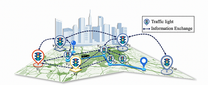
Figure 1: Decentralized traffic signal control system
图 1:分布式交通信号控制系统
相关文章的 Github 仓库位于 https://github.com/EEEEEclectic/traffic_signal_control。
Traffic Signal Control 交通信号控制
Effective traffic signal control in modern smart cities is a critical challenge due to the increasing complexity of urban traffic networks. Traffic signal control is often viewed as a complex networked system control problem, where interactions between traffic lights and road networks need to be dynamically managed and attaining controller adaptivity and scalability becomes a primary challenge [11].
现代智慧城市中有效的交通信号控制是一个关键挑战,因为城市交通网络的复杂性不断增加。交通信号控制通常被视为一个复杂的网络系统控制问题,其中交通灯和道路网络之间的交互需要动态管理,而实现控制器的适应性和可扩展性成为主要挑战[11]。
Given the interconnected dynamics of traffic signals and road infrastructure, MARL has emerged as a promising framework to address this challenge. MARL allows decentralized agents, such as traffic lights, to learn optimal control policies by interacting with their environment. However, existing MARL algorithms often fail to efficiently capture the spatial-temporal correlations among traffic signals, a crucial factor in improving the learning and decision-making capacity of decentralized agents.
鉴于交通信号和道路基础设施的相互动态关系,多智能体强化学习(MARL)已成为应对这一挑战的有前景的框架。MARL 允许交通灯等分布式智能体通过与环境的交互学习最优控制策略。然而,现有的 MARL 算法往往无法有效地捕捉交通信号之间的时空相关性,这是提高分布式智能体的学习和决策能力的一个关键因素。
In this project, we aim to evaluate centralized and decentralized control architecture by leveraging graph learning techniques, focusing on capturing the spatial-temporal correlations between traffic signals through effective information aggregation and message passing.
在这个项目中,我们旨在通过利用图学习技术评估集中式和分布式控制架构,重点关注通过有效的信息聚合和消息传递来捕捉交通信号之间的时空相关性。
Centralized vs Decentralized Reinforcement Learning
集中式与去中心化强化学习
Within multi-agent reinforcement learning, there are two main approaches: centralize, decentralized.
在多智能体强化学习中,主要有两种方法:集中式、分散式。
Under a centralized approach, a model used to output the next action for each agent utilizing all environment information, attempting to optimize for a global reward with observations across all agents.
在集中式方法下,使用一个模型来输出每个智能体的下一个动作,利用所有环境信息,试图通过跨所有智能体的观察来优化全局奖励。
Under a decentralize approach, each agent will have it’s own model, utilizing only local information of each agent to output the next action, and optimizes for a local reward, in an attempt to optimize for a global aggregate reward.
在分散式方法下,每个智能体都有自己的模型,仅利用每个智能体的局部信息来输出下一个动作,并优化局部奖励,试图优化全局总奖励。
Decentralized control offers significant advantages over centralized control in traffic management systems. In a decentralized approach, each agent communicates solely with its local neighbors, significantly reducing communication overhead and improving system scalability. This decentralised method is particularly well-suited for large-scale traffic networks where centralised aggregation can become a bottleneck.
分散式控制相比集中式控制,在交通管理系统中有显著优势。在分散式方法中,每个智能体仅与其局部邻居通信,显著减少了通信开销并提高了系统可扩展性。这种分散式方法特别适用于大规模交通网络,其中集中式聚合可能成为瓶颈。
A key insight supporting decentralized control in traffic networks is the natural decay of correlations with distance: as the road distance between traffic lights increases, their mutual influence diminishes. This spatial property means that focusing on local graph structures captures the most relevant information for decision-making, as traffic conditions at distant intersections have minimal impact on local traffic patterns. Consequently, agents can make robust decisions and collaborate effectively using primarily local information [Figure 2].
支持交通网络中分散控制的一个关键洞察是相关性的自然衰减与距离:随着交通灯之间道路距离的增加,它们之间的相互影响会减弱。这种空间特性意味着关注局部图结构可以捕捉到决策中最相关的信息,因为远处交叉口的交通状况对局部交通模式的影响最小。因此,代理可以利用主要局部信息做出稳健的决策并有效协作[图 2]。
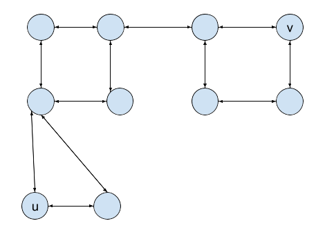
Figure 2: Traffic system, where each node is a traffic signal, and directed edges indicate lanes connecting traffic signals. Nodes u, v are far apart, and traffic signal actions of u,v will likely have little impact on one another.
图 2:交通系统,其中每个节点是一个交通信号灯,有向边表示连接交通信号灯的车道。节点 u 和 v 相距较远,u 和 v 的交通信号灯操作很可能对彼此影响不大。
Beyond the benefits of reduced information aggregation costs, decentralized control addresses another crucial challenge: the exponential growth of the action space in centralized systems as the traffic network scales. In centralized control, the complexity of the action space makes it increasingly difficult for a single agent to search effectively and find optimal policies. Decentralized control circumvents this limitation by distributing the decision-making process across multiple agents, each handling a manageable portion of the overall system.
除了减少信息聚合成本之外,去中心化控制还解决了另一个关键挑战:随着交通网络的扩展,集中式系统中的动作空间呈指数级增长。在集中式控制中,动作空间的复杂性使得单个智能体越来越难以有效地搜索并找到最优策略。去中心化控制通过将决策过程分布到多个智能体来规避这一限制,每个智能体负责处理系统整体中可管理的一部分。
数据
Commonly, traffic system information for traffic system tasks are configured in two types of files: route, network. The network file describes the entire traffic system network, assigning labels for each traffic signal, lane, and also how the entities interact with one another, such as which lanes are controlled by which traffic signals, or which lanes can you swap to from another lane. The default traffic light control configuration is also specified in the network file thus we can use the default policy in warmup phases to get the last k observations to capture the temporal correlation before transitioning to RL-based control.
通常,用于交通系统任务的交通系统信息配置在两种类型的文件中:路线、网络。网络文件描述了整个交通系统网络,为每个交通信号、车道分配标签,并指定实体之间的交互方式,例如哪些车道由哪些交通信号控制,或者哪些车道可以与其他车道交换。默认的交通灯控制配置也在网络文件中指定,因此我们可以在预热阶段使用默认策略获取最后 k 个观察结果,以捕获时间相关性,然后再过渡到基于强化学习的控制。
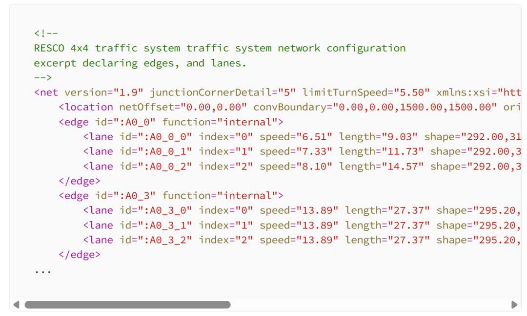
<!--
RESCO 4x4 traffic system traffic system network configuration
excerpt declaring edges, and lanes.
-->
<netversion="1.9"junctionCornerDetail="5"limitTurnSpeed="5.50"xmlns:xsi="http://www.w3.org/2001/XMLSchema-instance"xsi:noNamespaceSchemaLocation="http://sumo.dlr.de/xsd/net_file.xsd">
<locationnetOffset="0.00,0.00"convBoundary="0.00,0.00,1500.00,1500.00"origBoundary="0.00,0.00,1500.00,1500.00"projParameter="!"/>
<edgeid=":A0_0"function="internal">
<laneid=":A0_0_0"index="0"speed="6.51"length="9.03"shape="292.00,313.60 291.65,311.15 290.60,309.40 288.85,308.35 286.40,308.00"/>
<laneid=":A0_0_1"index="1"speed="7.33"length="11.73"shape="292.00,313.60 291.65,309.75 290.60,307.00 288.85,305.35 286.40,304.80"/>
<laneid=":A0_0_2"index="2"speed="8.10"length="14.57"shape="292.00,313.60 291.65,308.35 290.60,304.60 288.85,302.35 286.40,301.60"/>
</edge>
<edgeid=":A0_3"function="internal">
<laneid=":A0_3_0"index="0"speed="13.89"length="27.37"shape="295.20,313.60 294.70,305.50 293.60,300.00 292.50,294.50 292.00,286.40"/>
<laneid=":A0_3_1"index="1"speed="13.89"length="27.37"shape="295.20,313.60 295.20,286.40"/>
<laneid=":A0_3_2"index="2"speed="13.89"length="27.37"shape="295.20,313.60 295.70,305.50 296.80,300.00 297.90,294.50 298.40,286.40"/>
</edge>
...
The route file simulates traffic, detailing information about types of vehicles, and routes they take at each existing time step.
该路线文件模拟交通,详细说明了车辆类型以及它们在每个现有时间步所采取的路线。
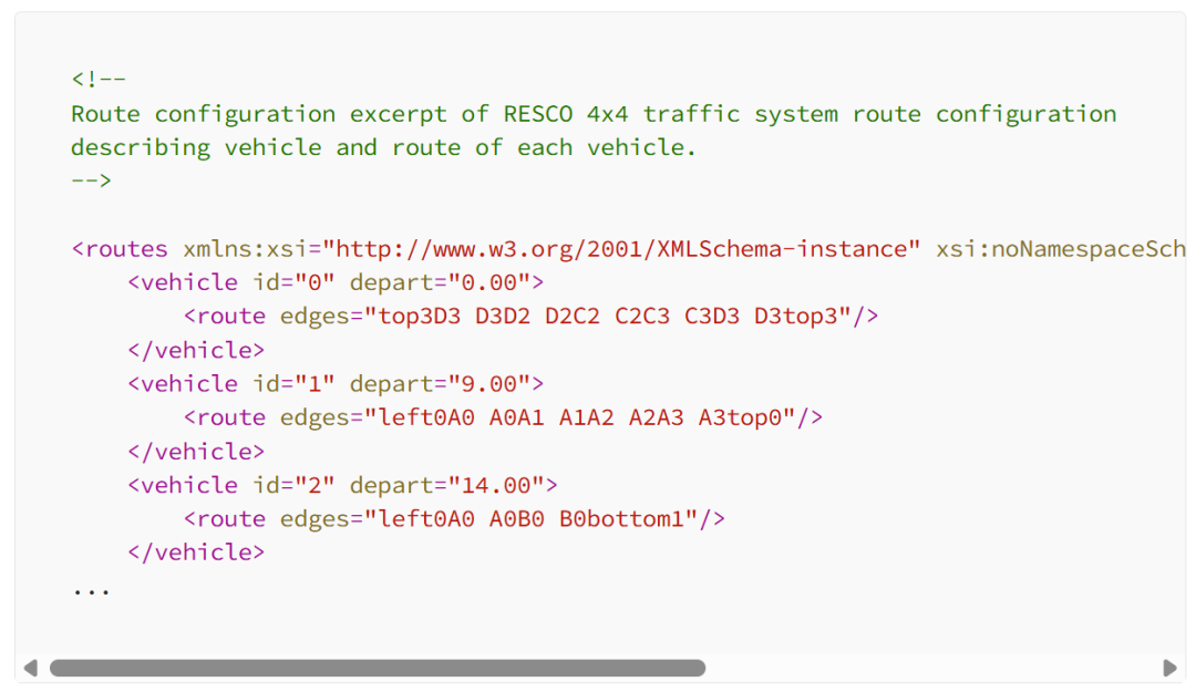
<!--
Route configuration excerpt of RESCO 4x4 traffic system route configuration
describing vehicle and route of each vehicle.
-->

<routesxmlns:xsi="http://www.w3.org/2001/XMLSchema-instance"xsi:noNamespaceSchemaLocation="http://sumo.dlr.de/xsd/routes_file.xsd">
<vehicleid="0"depart="0.00">
<routeedges="top3D3 D3D2 D2C2 C2C3 C3D3 D3top3"/>
</vehicle>
<vehicleid="1"depart="9.00">
<routeedges="left0A0 A0A1 A1A2 A2A3 A3top0"/>
</vehicle>
<vehicleid="2"depart="14.00">
<routeedges="left0A0 A0B0 B0bottom1"/>
</vehicle>
...
Together, the network and route configurations help describe both the traffic system network, and the simulated route of each vehicle within the system.
总之,网络和路线配置有助于描述交通系统网络以及系统内每辆车的模拟路线。
The default traffic light control configuration is also specified in the network file thus we can use the default policy in warmup phases to get the last k observations to capture the temporal correlation before transitioning to RL-based control.
网络文件中也指定了默认的信号灯控制配置,因此我们可以在预热阶段使用默认策略来获取最后 k 个观测结果,以捕捉在过渡到基于 RL 的控制之前的时序相关性。
SUMO-RL
We will utilize SUMO-RL for creating the environment and data necessary for tackling the traffic signal control problem, an open-source project (https://github.com/LucasAlegre/sumo-rl) designed to simulate traffic for reinforcement learning paradigms.
我们将使用 SUMO-RL 来创建解决交通信号控制问题所需的环境和数据,这是一个用于模拟强化学习范式的开源项目(https://github.com/LucasAlegre/sumo-rl)。
SUMO-RL provides a simple API, in setting the traffic system environment with the network and route configurations, and integrated with Open AI Gym, to more easily train, test algorithms and models in a reinforcement learning environment. SUMO-RL also provides both a centralized and decentralized multi-agent environment, allowing easy work in setting up the MARL for traffic system control task.
SUMO-RL 提供了一个简单的 API,用于设置交通系统环境,包括网络和路线配置,并与 Open AI Gym 集成,以便更轻松地在强化学习环境中训练、测试算法和模型。SUMO-RL 还提供了集中式和去中心化的多智能体环境,便于为交通系统控制任务设置 MARL。
import sumo_rl

# Simple setup using SUMO-RL to create reinforcement learning environment.
env = sumo_rl.parallel_env(net_file='nets/RESCO/grid4x4/grid4x4.net.xml',
                  route_file='nets/RESCO/grid4x4/grid4x4_1.rou.xml',
                  use_gui=True,
                  num_seconds=3600)
observations = env.reset()
# Simple to use SUMO-RL to generate environment to train/test.
while env.agents:
    actions = {agent: env.action_space(agent).sample() for agent in env.agents}  # this is where you would insert your policy
    observations, rewards, terminations, truncations, infos = env.step(actions)
问题陈述
The traffic signal control problem in SUMO-RL is modeled as a Markov Decision Process (MDP).
SUMO-RL 中的交通信号控制问题被建模为马尔可夫决策过程(MDP)。
More specifically: 更具体地说:
State (S): Each traffic signal is treated as an individual agent. The state of a traffic signal is defined as the last k observations of nodes in the (local) graph. The observations represent the lane density ∈ [0, 1] and queue ∈ [0, 1] of vehicles in the incoming lanes of the intersection. The detail will be given later in the Data Preprocessing section.
状态(S):每个交通信号被视为一个独立的智能体。交通信号的状态定义为(局部)图中节点的最后 k 次观测结果。观测结果表示交叉路口入口车道的车辆密度 ∈ [0, 1] 和排队 ∈ [0, 1]。详细内容将在数据预处理部分给出。
Action (A): The action set for each agent consists of all possible green light configurations for the respective intersection. The number of possible configurations depends on the number of lanes at the intersection.
动作(A):每个智能体(agent)的动作集由相应交叉口的全部可能的绿灯配置组成。可能的配置数量取决于交叉口的车道数量。
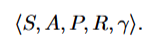
Reward (R): SUMO-RL provides an interface to define custom reward functions tailored to the objectives of the traffic signal control problem. The reward at each agent i at time step τ is defined as:
奖励(R):SUMO-RL 提供了一个接口来定义针对交通信号控制问题目标的定制奖励函数。在智能体 i 在时间步τ的奖励定义为:
to balance traffic congestion and trip delay via ω where:
通过ω来平衡交通拥堵和行程延误:
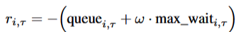
queue_i,τ: The sum of normalized queue values for all incoming lanes at traffic signal i. The queue for each lane is defined as:
queue_i,τ:交通信号 i 处所有进入车道的归一化队列值的总和。每个车道的队列定义为:
The queue value for each lane is clipped to a maximum of 1.
每个车道的队列值被裁剪到最大值为 1。
max_wait_i,τ: The normalized maximum cumulative waiting time of the first vehicles in each incoming lane at traffic signal i. This is calculated as:
max_wait_i,τ:交通信号 i 处每个进入车道的首批车辆的归一化最大累积等待时间。该值计算如下:

γ: A weighting factor to balance the impact of queue length and cumulative waiting time in the reward function.
γ:用于在奖励函数中平衡队列长度和累积等待时间影响的权重因子。
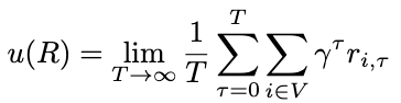
From a global perspective, the traffic signal control problem is a cooperative game where all agents aim to optimize a shared global reward. The global reward utility function is defined as:
从全局角度来看,交通信号控制问题是一个合作博弈,其中所有智能体都旨在优化一个共享的全局奖励。全局奖励效用函数定义如下:
This setup enables a decentralized multi-agent reinforcement learning framework, where each traffic signal optimizes its actions to improve traffic flow.
该设置实现了一个去中心化的多智能体强化学习框架,其中每个交通信号灯都优化其动作以改善交通流量。
数据预处理
Since our model utilizes graph representation as input, we will need to transform the SUMO-RL representation of the traffic signal system into a graph representation with nodes and edges, with feature vectors.
由于我们的模型使用图表示作为输入,因此我们需要将 SUMO-RL 交通信号系统表示转换为具有节点和边的图表示,并带有特征向量。
Graph Representation 图表示
SUMO-RL represents the traffic signal system as a dictionary of traffic signals, where each traffic signal object holds observable information, such as the state of the traffic light, a list of incoming lane Ids, and a list of outgoing lane Ids.
SUMO-RL 将交通信号系统表示为一个交通信号灯的字典,其中每个交通信号灯对象包含可观察的信息,例如交通灯的状态、传入车道的 ID 列表和传出车道的 ID 列表。
# SUMO-RL represents traffic system as dictionary of traffic signals,
# mapping traffic signal id to TrafficSignal object
classSumoEnvironment(gym.Env):
def__init__(...):
      ...
self.traffic_signals = {
ts: TrafficSignal(
self,
                    ts,
self.delta_time,
self.yellow_time,
self.min_green,
self.max_green,
self.begin_time,
self.reward_fn,
                    conn,
                )
for ts inself.ts_ids
            }
      ...
# Each TrafficSignal objects holds information about the lanes it manages,
# such as list of incoming lanes, and outgoing lanes.
# Also providing API to access aggregated traffic information (i.e. congestion, density).
classTrafficSignal:
def__init__(self,
        env,
ts_id: str,
delta_time: int,
yellow_time: int,
min_green: int,
max_green: int,
begin_time: int,
reward_fn: Union[str, Callable],
        sumo,
):
    ...
self.id = ts_id
self.env = env
self.delta_time = delta_time
self.yellow_time = yellow_time
self.min_green = min_green
self.max_green = max_green
self.green_phase = 0
self.is_yellow = False
self.time_since_last_phase_change = 0
self.next_action_time = begin_time
self.last_measure = 0.0
self.last_reward = None
self.reward_fn = reward_fn
self.sumo = sumo
    ...
# Get total waiting time per lane.
defget_accumulated_waiting_time_per_lane(self) -> List[float]: ...
# Get maximum waiting time per lane.
defget_max_cumulative_waiting_time_of_the_first_vehicles_per_lane(self) -> List[float]: ...
Utilizing traffic signal information, we generate a directed graph representation. Each node is a traffic signal, identifiable with a unique traffic signal Id, and each directed edge between two nodes exist if there exists at least one lane connecting the two nodes [Figure 4]. Since a lane can serve as either an entry or exit point for the traffic system, it is possible to encounter dangling edges with no associated starting or ending nodes. To address this, we incorporate virtual nodes into the graph to represent incoming and outgoing lanes. These virtual nodes have trivial observations, where all density and waiting time features are set to zero. However, they retain critical graph structural information about the traffic network, ensuring an accurate representation of its topology.
利用交通信号信息,我们生成了一个有向图表示。每个节点是一个交通信号,可以用唯一的交通信号 ID 来识别,并且两个节点之间存在有向边,当且仅当两个节点之间存在至少一条车道连接时[图 4]。由于车道可以作为交通系统的入口或出口,因此可能会遇到没有关联的起始或结束节点的悬空边。为了解决这个问题,我们在图中加入了虚拟节点来表示进出车道。这些虚拟节点的观察值是平凡的,其中所有密度和等待时间特征都设置为 0。但是它们保留了关于交通网络的关键图结构信息,确保了其拓扑结构的准确表示。
defconstruct_graph_representation(ts_list):
'''
    Build graph representation of TrafficSignal traffic system.
    Returns:
        ts_idx: mapping of TrafficSignal id to associated node index.
        num_nodes: total number of nodes in graph.
        lanes_index: mapping of lane id to associated edge index in adj_list.
        adj_list (np.array): Adjancency list of size [|E|, 2].
        incoming_lane_ts (list[int]): containing the indices of traffic signals connecting to incoming virtual nodes.
        outgoing_lane_ts (list[int]): containing the indices of traffic signals connecting to outgoing virtual nodes.
    Args:
        ts_list (list[TrafficSignal]): list of TrafficSignal to build graph representation for.
    '''
# collect traffic signal ids
# sort_ts_func = lambda ts: ts.id
# ts_idx = {ts.id: i for i, ts in enumerate(sorted(ts_list, key=sort_ts_func))}
    ts_idx = {ts.id: i for i, ts inenumerate(ts_list)}
# collect all lane ids
    lanes = [ts.lanes + ts.out_lanes for ts in ts_list]
    lanes = [lane for ln in lanes for lane in ln]
    lanes_index = {ln_id: i for i, ln_id inenumerate(sorted(set(lanes)))}
# calculate all ts_start, ts_end for all lanes
    adj_list = [[-1for _ inrange(2)] for _ inrange(len(lanes_index))]
# fill with additional dummy nodes
for ts in ts_list:
        ts_id = ts_idx[ts.id]
for in_edge in ts.lanes:
            in_edge_idx = lanes_index[in_edge]
            adj_list[in_edge_idx][1] = ts_id
for out_edge in ts.out_lanes:
            out_edge_idx = lanes_index[out_edge]
            adj_list[out_edge_idx][0] = ts_id
    incoming_indx = len(ts_idx)
    outgoing_indx = incoming_indx + 1
    incoming_lane_ts = []
    outgoing_lane_ts = []
# for unassigned positions, add dummy nodes
for lane in adj_list:
if lane[0] == -1or lane[1] == -1:
if lane[1] == -1:
                lane[1] = outgoing_indx
                outgoing_lane_ts.append(lane[0])
else:
                lane[0] = incoming_indx
                incoming_lane_ts.append(lane[1])
    num_nodes = outgoing_indx + 1
return ts_idx, num_nodes, lanes_index, np.array(adj_list), incoming_lane_ts, outgoing_lane_ts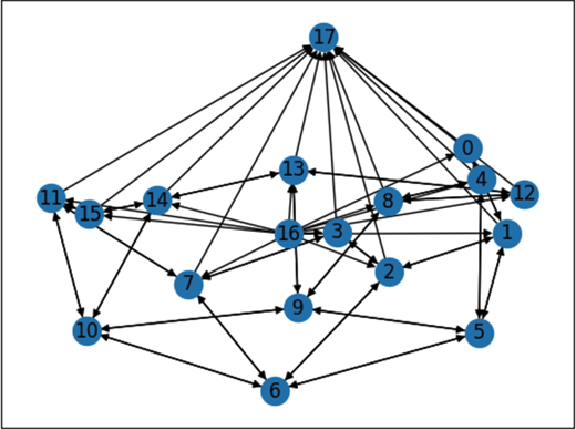
Figure 4: Graph representation of 4x4 traffic signal system
图 4:4x4 交通信号系统的图表示
Action/State Space Representation
动作/状态空间表示
1. State Space: As described in the problem statement, the state space is defined as the last k observations of nodes in the graph (local graph in the case of decentralized control). The observations represent the lane density ∈ [0, 1] and queue ∈ [0, 1] of vehicles in the incoming lanes of the intersection.
1. 状态空间:如问题陈述所述,状态空间定义为图中节点的最后 k 个观察值(在去中心化控制的情况下为局部图)。观察值表示交叉路口 incoming lanes 中车辆的密度 ∈ [0, 1] 和队列 ∈ [0, 1]。
Lane Density: Computed as the number of vehicles divided by the maximum number of vehicles that can fit in the lane.
车道密度:计算为车道内车辆数量除以车道能容纳的最大车辆数。
Queue: Computed as the number of halted vehicles divided by the maximum number of vehicles that can fit in the lane.
队列:计算为停止的车辆数量除以车道能容纳的最大车辆数。
2. Observation and Action Space Standardization: To ensure the model is generalizable and capable of handling intersections with varying numbers of lanes, both the observation space and action space are standardized:
2. 观测和动作空间标准化:为确保模型具有泛化能力并能够处理车道数量不同的交叉口,观测空间和动作空间均进行了标准化:
Observation Space: Padded to the maximum number of lanes across all traffic signals.
观测空间:填充到所有交通信号灯中车道数量的最大值。
defprocess_observation_buffer_with_graph(observation_buffer, ts_idx, max_lanes, num_nodes):
"""
    Process the observation buffer into a uniform tensor suitable for model input
    Args:
        observation_buffer (list[dict]): Observation buffer where each entry is a dict of
                                         {ts_id: observation},
                                         and observation contains:
                                         {
                                             "density": np.array([...]), length=num_lanes
                                             "queue": np.array([...])
                                         }.
        ts_idx (dict): Mapping of TrafficSignal id to node index from `construct_graph_representation`.
        max_lanes (int): Maximum number of lanes across all traffic signals.
        num_nodes (int): including virtual nodes incoming/outgoing_index
    Returns:
        np.ndarray: shape [num_timesteps, num_nodes, feature_size]
    """
    num_timesteps = len(observation_buffer)
#num_traffic_signals = len(ts_idx)
    feature_size = 2 * max_lanes  # density and queue for each lane
    processed_buffer = np.zeros((num_timesteps, num_nodes, feature_size), dtype=np.float32)
for t_idx, timestep inenumerate(observation_buffer):
for ts_id, obs in timestep.items():
            ts_index = ts_idx[ts_id]
# Pad density and queue
            padded_density = np.pad(obs["density"], (0, max_lanes - len(obs["density"])), mode="constant")
            padded_queue = np.pad(obs["queue"], (0, max_lanes - len(obs["queue"])), mode="constant")
# Combine features
            processed_buffer[t_idx, ts_index, :] = np.concatenate([padded_density, padded_queue])
return processed_buffer
Action Space: Padded to the maximum number of green light phases across all traffic signals. To ensure our model will output valid green phase for each traffic signal, we need masking out the invalid actions by adding a very large negative number to the action logits outputted from the model.
动作空间:填充到所有交通信号灯的最大绿灯相位数。为了确保我们的模型将为每个交通信号灯输出有效的绿灯相位,我们需要通过在模型输出的动作 logits 上添加一个非常大的负数来屏蔽无效的动作。
defcreate_action_mask(num_nodes, max_green_phases, valid_action_counts):
"""
    Create a mask for traffic node actions, where each node may have a different number of valid actions.
    The last two nodes are virtual nodes and have no valid actions.
    Args:
        num_nodes (int): Total number of nodes, including traffic nodes and virtual nodes.
        max_green_phases (int): Maximum number of actions across all nodes.
        valid_action_counts (list[int]): List of valid action counts for each traffic node.
    Returns:
        torch.Tensor: A binary mask of shape (num_nodes, max_green_phases).
    """
    mask = torch.zeros((num_nodes, max_green_phases), dtype=torch.float32)
# Assign valid actions for each node
for i, count inenumerate(valid_action_counts):
        mask[i, :count] = 1.0
return mask
Prior Work 以往研究
Our approach builds upon existing research in centralized and decentralized traffic signal control, i.e. single-agent and multi-agent reinforcement learning (MARL) frameworks and leverage different graph encoders, such as DCRNN, SA-GNN, DTLight etc. to perform representation learning which effectively capturing spatiotemporal correlations in the traffic network.
我们的方法建立在现有的集中式和分布式交通信号控制研究之上,即单代理和多代理强化学习(MARL)框架,并利用不同的图编码器,如 DCRNN、SA-GNN、DTLight 等,进行表示学习,有效地捕捉交通网络中的时空相关性。
Diffusion Convolutional Recurrent Neural Network (DCRNN)
扩散卷积循环神经网络(DCRNN)
The DCRNN model leverages a diffusion convolution [1] layer to capture spatial correlations within the traffic network. DCRNN utilizes a recurrent architecture, utilizing a bidirectional diffusion process to capture the influence from both upstream and downstream traffic flow [8, Figure 5].
DCRNN 模型利用扩散卷积层[1]来捕获交通网络内的空间相关性。DCRNN 采用循环架构,利用双向扩散过程来捕获上游和下游交通流的影响[8,图 5]。
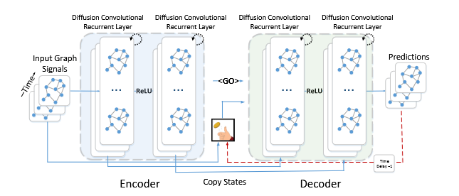
Figure 5: DCRNN architecture
图 5:DCRNN 架构
DCRNN indicates to be a strong architecture in diffusing and integrating temporal information, and can be utilized in both a centralized, and decentralized setting. We will use centralized DCRNN model as our baseline, and compare the performance metrics across other decentralized implementation.
DCRNN 是一种在扩散和整合时间信息方面表现强大的架构,并且可以在集中式和分散式环境中使用。我们将使用集中式 DCRNN 模型作为我们的基线,并比较其他分散式实现中的性能指标。
SA-GNN
In this approach, each agent only exchanges information with its immediate neighbors, and information is recursively aggregated to capture both local and multi-hop (K-hop) dependencies [2, Figure 6].
在这种方法中,每个智能体仅与其直接邻居交换信息,并且信息会递归地聚合以捕获局部和多跳(K 跳)依赖关系[2,图 6]。
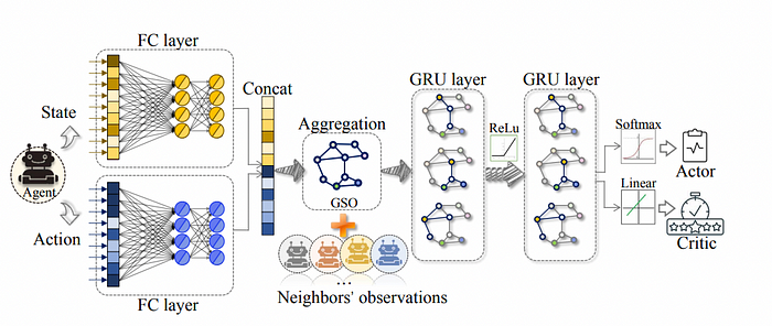
Figure 6: SA-GNN architecture.
图 6:SA-GNN 架构。
After aggregating information from direct neighbors, each agent constructs a local graph. As the graph depth or the number of hops increases, the local graph incorporates delayed information from farther neighbors. Specifically, the local graph constructed on-the-fly contains t−k information from k-hop neighbors, as each agent only communicates with its direct neighbors. This design reflects a tradeoff between communication cost and the timeliness of the information in the local graph. Increasing the number of hops provides a broader view of the traffic network but at the expense of relying on older information from distant nodes.
在聚合来自直接邻居的信息后,每个智能体构建一个局部图。随着图深度或跳数的增加,局部图会包含来自更远邻居的延迟信息。具体来说,智能体实时构建的局部图包含了 k 跳邻居的 t-k 信息,因为每个智能体只与其直接邻居通信。这种设计体现了通信成本和局部图中信息时效性之间的权衡。增加跳数可以提供更广泛的交通网络视图,但代价是依赖来自远距离节点的较旧信息。
After building the local graph, SA-GNN will use the a different diffusion process as DCRNN on the local graph to get the final graph representation used for decision making.
在构建局部图后,SA-GNN 将使用与 DCRNN 不同的扩散过程在局部图上得到最终用于决策的图表示。
DTLight
DTLight takes a unique approach compared to models like DCRNN or SA-GNN by utilizing a transformer architecture to determine the actions of each agent at every time step in a centralized manner [6, Figure 7]. In its implementation, the transformer acts like an undirected fully connected graph, where the attention matrix represents the attention values between traffic signals in the system.
DTLight 与 DCRNN 或 SA-GNN 等模型相比,采用了一种独特的方法,通过使用 Transformer 架构以集中方式确定每个智能体在每个时间步长的动作 [6, 图 7]。在其实现中,Transformer 像一个无向全连接图,其中注意力矩阵表示系统中的交通信号之间的注意力值。
However, a key limitation of DTLight is that, due to its reliance on the transformer architecture, it assumes a fully connected graph structure for the input. This fails to capture the spatial and structural characteristics inherent to traffic networks, which are often sparse and have well-defined local connectivity patterns.
然而,DTLight 的一个关键局限性在于,由于其依赖于 Transformer 架构,它假设输入为全连接图结构。这无法捕捉交通网络固有的空间和结构特征,这些网络通常是稀疏的,并且具有明确定义的局部连接模式。
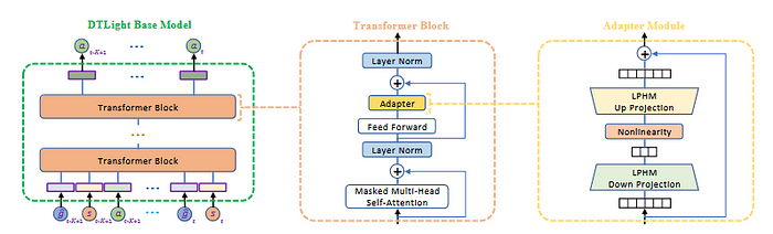
Figure 7: DTLight architecture
图 7:DTLight 架构
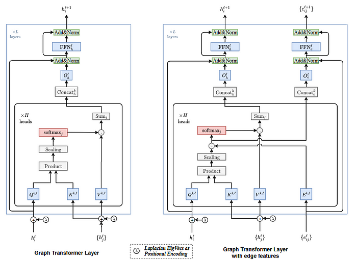
In contrast, we propose the use of a graph-transformer model, which differs fundamentally from a pure transformer. In a graph-transformer, the layer operates on each node and its immediate neighbors, allowing for variability in the number of neighbors across nodes. This creates a localized attention mechanism that focuses on a node’s neighborhood rather than considering all nodes in the graph simultaneously [7, Figure 8]. Additionally, graph-transformer layers leverage positional encoding to encode the relative position of each node within the graph. This feature enhances the model’s ability to distinguish between different inputs and better preserves the structural information of the traffic network.
相比之下,我们提出了使用图转换器模型,这与纯转换器有根本区别。在图转换器中,层对每个节点及其直接邻居进行操作,允许节点邻居数量的变化。这创建了一种局部注意力机制,该机制专注于节点的邻域,而不是同时考虑图中的所有节点[7, 图 8]。此外,图转换器层利用位置编码来编码每个节点在图中的相对位置。这一特性增强了模型区分不同输入的能力,并更好地保留了交通网络的结构信息。
Our Best Model: Decentralized Transformer-based Traffic Signal Control
我们的最佳模型:基于 Transformer 的去中心化交通信号控制
Unlike previous work, we also try to decouple the modelling of spatial and temporal correlation separately. Specifically, we first use recurrent models to capture temporal correlations and compress temporal information into a compact representation. This temporal representation is then passed into a graph-transformer model, which focuses on capturing the spatial correlations unique to the given traffic network, which shows robust experimentation outcome.
与之前的工作不同,我们还尝试将空间和时间的建模分开。具体来说,我们首先使用循环模型来捕获时间相关性,并将时间信息压缩成紧凑的表示。然后将这种时间表示传递到图转换器模型中,该模型专注于捕获给定交通网络特有的空间相关性,实验结果表明其具有鲁棒性。
Local Information: 局部信息
For each agent, we dynamically construct a local k-hop graph. Since the traffic network is directed, both upstream and downstream traffic flows are considered. This ensures that the agent has a comprehensive understanding of its current state, enabling more robust decision-making. The k-hop local graph includes both incoming and outgoing neighbors, providing a holistic view of the surrounding traffic flow.
对于每个智能体,我们动态构建一个局部 k 跳图。由于交通网络是定向的,因此考虑了上游和下游的交通流。这确保了智能体对其当前状态的全面了解,从而能够做出更稳健的决策。k 跳局部图包括传入和传出的邻居,提供了周围交通流的整体视图。
To incorporate temporal context, each node in the local graph retains its past observations. This allows the input to encapsulate both spatial and temporal information, ensuring the model captures spatio-temporal correlations effectively for improved traffic signal control.
为了结合时间上下文,局部图中的每个节点都保留其过去的观察结果。这使得输入能够封装空间和时间信息,确保模型能够有效地捕捉时空相关性,从而改进交通信号控制。
defcreate_local_graph(self, ts_id, max_lane):
"""
        Create a local graph for the given traffic signal, considering both directions.Args:
            ts_id (str): Traffic signal ID.
            max_lane (int): Maximum number of lanes to pad density/queue.
        Returns:
            subgraph_features (torch.Tensor): Features for the local subgraph nodes.
            subgraph_nodes (torch.Tensor): Indices of nodes in the subgraph.
            subgraph_edge_index (torch.Tensor): Edge index of the subgraph.
        """
        node_index = self.ts_indx[ts_id]
        st_nodes, st_edge_index, _, _ = torch_geometric.utils.k_hop_subgraph(
            node_idx=node_index, num_hops=self.hops, edge_index=self.edge_index, relabel_nodes=False, flow="source_to_target"
        )
        ts_nodes, ts_edge_index, _, _ = torch_geometric.utils.k_hop_subgraph(
            node_idx=node_index, num_hops=self.hops, edge_index=self.edge_index, relabel_nodes=False, flow="target_to_source"
        )
        subgraph_nodes = torch.cat((st_nodes, ts_nodes)).unique(sorted=False)
        subgraph_edge_index = torch.cat((st_edge_index, ts_edge_index), dim=1).unique(dim=1)
        nodes_mapping = {node.item(): i for i, node inenumerate(subgraph_nodes)}
# Map edges using the node mapping
        subgraph_edge_index = torch.stack([
            torch.tensor([nodes_mapping[u.item()] for u in subgraph_edge_index[0]]),
            torch.tensor([nodes_mapping[v.item()] for v in subgraph_edge_index[1]])
        ], dim=0)
# Aggregate features for the combined subgraph
        idx_to_ts_id = {v: k for k, v in self.ts_indx.items()}
# create placeholder for subgraph_features: shape (num_timesteps, num_nodes, feature_size)
        subgraph_features = torch.zeros((self.k, len(subgraph_nodes), 2*max_lane), dtype=torch.float32)
for local_idx, node_idx inenumerate(subgraph_nodes):
            ts_id = idx_to_ts_id.get(node_idx.item(), None)
if ts_id isNone:
continue
            node_obs = self.last_k_observations[ts_id]
for t, obs inenumerate(node_obs):
# Pad density and queue features
                density = torch.tensor(obs["density"], dtype=torch.float32)
                queue = torch.tensor(obs["queue"], dtype=torch.float32)
                padded_density = torch.nn.functional.pad(density, (0, max_lane - len(density)))
                padded_queue = torch.nn.functional.pad(queue, (0, max_lane - len(queue)))
# Concatenate density and queue features
                subgraph_features[t, local_idx, :] = torch.cat((padded_density, padded_queue))
return subgraph_features, subgraph_nodes, subgraph_edge_index
Policy Model 策略模型
For our decentralized approach, we will define a graph-transformer based approach, utilizing LSTM for preprocessing, transformer convolution layers, with skip connections, and a final projection head for outputting the next agent action [5, Figure 9].
对于我们的分布式方法,我们将定义一个基于图转换的方法,利用 LSTM 进行预处理,使用带有跳跃连接的 Transformer 卷积层,以及一个最终投影头来输出下一个智能体动作[5, 图 9]。
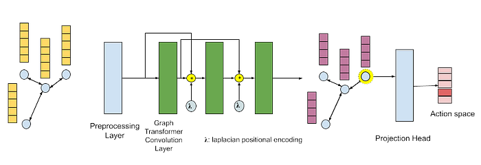
Figure 9: Architecture of model. Includes preprocessing layer, and graph-transformer convolution layers, utilizing a projection head to determine agent action.
图 9:模型架构。包括预处理层,以及使用投影头确定智能体动作的图 Transformer 卷积层。
1. Preprocessing Layer 预处理层
As discussed above, we use recurrent model to get the representation encoding the temporal information. Here we used LSTM to capture temporal correlation.
如上所述,我们使用循环模型来获取编码时间信息的表示。这里我们使用 LSTM 来捕获时间相关性。
from torch.nn import LSTM, LeakyReLU

classGraphTransformerNetwork(torch.nn.Module):
def__init__(self, ts_map, traffic_system, args):
        ...
        self.preprocess = LSTM(input_size=self.input_features, hidden_size=self.hidden_features, num_layers=self.num_layers)
        ...
2. Graph-Transformer Convolution
2. 图 Transformer 卷积
The graph-transformer layers perform diffusion convolution for message passing, to diffuse and share information between traffic signals within the subgraph. As input, we will concatenate positional encoding information, with Laplacian positional encoding [Figure 9]. Laplacian positional encoding provides robust positional information of data to provide more information for attention mechanism within the transformer layer.
图形转换器层执行扩散卷积以进行消息传递,以在子图内的交通信号之间扩散和共享信息。作为输入,我们将连接位置编码信息,以及拉普拉斯位置编码[图 9]。拉普拉斯位置编码为数据提供稳健的位置信息,为转换器层内的注意力机制提供更多信息。
defget_laplacian_eigenvecs(G):
    laplacian = nx.laplacian_matrix(G).toarray()
    eigenvals, eigenvecs = np.linalg.eig(laplacian)
return laplacian, eigenvals, eigenvecs

    ...
# eigenvecs are stacked, such that the ith column is the ith eigenvector
# We take the ith row to get the positional encoding for the ith node.
    pos = np.take(eigenvecs, indices.cpu().numpy(), axis=0)
Furthermore, we will utilize skip connections between convolution layers to help integrate previous embedding to help generate the embedding for the next layer. To avoid issues with over-smoothing, where the size of the local subgraph, and the deepness of the model can lead to convergence of node embeddings, we utilize both skip connections, and adjustable hyper-parameter to determine number of layers of diffusion convolution.
此外,我们将利用卷积层之间的跳跃连接来帮助整合先前的嵌入,以帮助生成下一层的嵌入。为了避免过度平滑问题,其中局部子图的大小和模型的深度可能导致节点嵌入收敛,我们利用跳跃连接和可调节的超参数来确定扩散卷积的层数。
from torch.nn import Linear, LeakyReLU

classGraphTransformerNetwork(torch.nn.Module):
...
defforward(self, node_features, edge_index, agent_index, subgraph_indices):
'''
        Args:
        * node_features: node features
        * edge_index: edge index describing graph
        * agent_index: agent to generate action for
        * subgraph_indices: list of node indices used in subgraph to add positional encoding
        '''
        x = node_features.float()
        ...

# Get Laplacian positional encoding for each node.
        pos = np.take(self.eigenvecs, subgraph_indices.cpu().numpy(), axis=0)
        pos = torch.tensor(pos, dtype=torch.float32)
if pos.shape[0] != x.shape[0]:
            pos = torch.nn.functional.pad(
                pos, (0, 0, 0, x.shape[0] - pos.shape[0]))
        prev = None
for layer in self.layers:
            temp = x
# Skip connection to concatenate embeddings of previous layer.
if prev isnotNone:
                x = torch.cat([x, prev], dim=1)
            prev = temp
# Add positional encoding.
            x = torch.cat([x, pos], dim=1)
            x = layer(x, edge_index)

        ...
For the diffusion convolution process, we will utilize graph-transformer layer, as described in PyTorch Geometric, the next node embedding is calculated via:
对于扩散卷积过程,我们将利用图形转换器层,如 PyTorch Geometric 中所述,下一个节点嵌入通过以下方式计算:
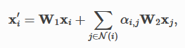
with attention calculated with:
注意力计算为:
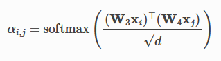
,where we utilize the node and it’s neighbors to calculate an attention matrix, which is then used to determine which neighboring nodes should have more emphasis in the resulting embedding [9]. Graph-transformers prove to be strong mechanism in providing attention mechanism to graph input.
我们利用节点及其邻居来计算注意力矩阵,该矩阵用于确定在结果嵌入中哪些相邻节点应具有更多权重[9]。图 Transformer 被证明是向图输入提供注意力机制的有效机制。
from torch.nn import Linear, LeakyReLU

classTransformerBlock(torch.nn.Module):
# Transformer block to easier build overall GraphTransformerNetwork
def__init__(self, in_channels, out_channels, heads=4, dropout=0.0):
super(TransformerBlock, self).__init__()
        self.transformer = TransformerConv(
            in_channels=in_channels, out_channels=out_channels, heads=heads, dropout=dropout)
        self.norm = BatchNorm1d(num_features=out_channels)
        self.relu = LeakyReLU()
        self.proj = Linear(in_features=heads*out_channels,
                           out_features=out_channels)
defforward(self, x, edge_index):
        x = self.transformer(x, edge_index)
        x = self.proj(x)
        x = self.norm(x)
        x = self.relu(x)
return x
classGraphTransformerNetwork(torch.nn.Module):
def__init__(self, ts_map, traffic_system, args):
        ...
# Add Transformer layers
        self.layers = ModuleList()
# Add self.eigenvec_len to account for positional encoding size.
        self.layers.append(TransformerBlock(in_channels=self.hidden_features+self.eigenvec_len,
                           out_channels=self.hidden_features, heads=4, dropout=self.dropout))
# Add prev to account for skip connection size.
        prev = self.hidden_features
for _ inrange(self.num_layers-2):
            self.layers.append(TransformerBlock(in_channels=self.hidden_features+prev +
                               self.eigenvec_len, out_channels=self.hidden_features, heads=4, dropout=self.dropout))
            prev = self.hidden_features
        self.layers.append(TransformerConv(in_channels=self.hidden_features+prev +
                           self.eigenvec_len, out_channels=self.hidden_features, heads=1, dropout=self.dropout))
        ...
3. Projection Head 投影头
The projection head will take the final embedding of the target agent from graph transformer as input, and using MLP layer to finally output the logits for all possible actions. To ensure we only sample valid actions, we need to apply the mask to the action logits.
投影头将图 Transformer 的目标代理的最终嵌入作为输入,并使用 MLP 层最终输出所有可能动作的对数概率。为了确保我们只采样有效动作,我们需要将掩码应用于动作对数概率。
from torch.nn import Linear, LeakyReLU

classGraphTransformerNetwork(torch.nn.Module):
def__init__(self, ts_map, traffic_system, args):
        ...
# Add projection head for classification
        proj_head = []
for _ inrange(self.num_proj_layers-1):
            proj_head.append(
                Linear(in_features=self.hidden_features, out_features=self.hidden_features))
            proj_head.append(LeakyReLU())
        proj_head.append(Linear(in_features=self.hidden_features,
                         out_features=self.output_features))
        self.proj_head = Sequential(*proj_head)
        self.softmax = LogSoftmax()
        ...

defforward(self, node_features, edge_index, agent_index, subgraph_indices):
'''
        Args:
        * node_features: node features
        * edge_index: edge index describing graph
        * agent_index: agent to generate action for
        * subgraph_indices: list of node indices used in subgraph to add positional encoding
        '''

        ...

# Extract embeddings for target node as input into projection head.
# Resulting output will be probabilities for the action that should be taken for the agent.
# Apply masking to only allow valid actions.
        local_agent_idx = (subgraph_indices == agent_index).nonzero(as_tuple=True)[0].item()
        logits = self.proj_head(x[local_agent_idx])
        logits = logits + (1 - self.mask[agent_index]) * -1e9
return logits
Experiments & Analysis 实验与分析
In our experimentation, we choose centralized DCRNN as our baseline, and compare with decentralized DCRNN and transformer model, we used policy gradient method as our learning algorithm.
在我们的实验中,我们选择集中式 DCRNN 作为我们的基线,并与去中心化 DCRNN 和 Transformer 模型进行比较,我们使用了策略梯度方法作为我们的学习算法。
We will show the details of training process for decentralized transformer model, and the others will be similar.
我们将展示去中心化 Transformer 模型的训练过程细节,其他部分也类似。
Because of decentralized nature, we will have separate models for each agent.
由于去中心化的特性,我们将为每个智能体设置单独的模型。
# Agent class to hold dictionary mapping each agent id to associated policy model.
classPGMultiAgent:
def__init__(self, ts_indx, edge_index, num_nodes, k, hops, model_args, device, gamma=0.99, lr=1e-4):
        self.models = {}
        self.optimizers = {}
        self.ts_indx = ts_indx
        self.num_nodes = num_nodes
        self.edge_index = edge_index  # [2, |E|]
        self.device = device
        self.gamma = gamma
        self.lr = lr
        self.k = k
        self.hops = hops
for ts_id in ts_indx.keys():
            self.models[ts_id] = PolicyNetwork(model_args).to(device)
            self.optimizers[ts_id] = optim.Adam(self.models[ts_id].parameters(), lr=lr)
        self.last_k_observations = {ts: [] for ts in ts_indx.keys()}
        self.no_op = {ts: 0for ts in ts_indx.keys()}
During training, we will keep track of the last k observations. When we enter the new episode, we will start with the warmup phase and using the default traffic signal control policy defined in the network file, after getting the new observation, we update the last k observations buffer. After the buffer is full, we can transition to RL control. Each agent will build their local graph based on current last k observations, passing through the model and sample actions from the output logits, keeping track of the rewards and action log-probability on the fly, and after one episode truncates, we will use the policy gradient learning algorithm to update the policy and then continue the next episode.
在训练过程中,我们将跟踪最后 k 个观察结果。当我们进入新的回合时,我们将开始预热阶段,并使用网络文件中定义的默认交通信号控制策略,在获得新的观察结果后,我们将更新最后 k 个观察结果缓冲区。当缓冲区满后,我们可以过渡到强化学习控制。每个智能体将根据当前的最后 k 个观察结果构建本地图,通过模型并从输出 logits 中采样动作,实时跟踪奖励和动作 log 概率,在一个回合结束时,我们将使用策略梯度学习算法来更新策略,然后继续下一个回合。
# Train agent with environment and number episode
deftrain(self, env, num_episodes):

      ...
      done = False
      it = 0
whilenot done:
# Warmup phase with default traffic light control
if it < self.k:
            obs, _, _, _, _ = env.step(self.no_op)  # Run default traffic light control
            self.update(obs)
            it += 1
continue
# RL control starts after warmup
if it == self.k:
          sumo_env.fixed_ts = False# Switch to RL control
for _, ts in sumo_env.traffic_signals.items():
            ts.run_rl_agents()  # Activate RL agents
for agent_name in env.agents:
          agent_idx = self.ts_indx[agent_name]
# Create local graph
          agents_features, subgraph_nodes, subgraph_edge_index = self.create_local_graph(
              agent_name, self.ts_indx, self.edge_index, self.hops, max_lanes
          )
# Run policy model for each agent and gather action logits.
# Uses generated probabilities to determine action for each agent.
          model = self.models[agent_name]
          logits = model(agents_features, subgraph_edge_index, agent_idx, subgraph_nodes)
          dist = torch.distributions.Categorical(logits=logits)
          action = dist.sample()
          actions[agent_name] = action.item()
          log_prob = dist.log_prob(action)
          agent_experiences[agent_name]['log_probs'].append(log_prob)

# Step the environment
          observations, rewards, terminations, truncations, infos = env.step(actions)
          self.update(obs)
      ...
Performance Metrics 性能指标
To evaluate performance, we record both system-level and agent-level metrics for each time step across all episodes. This results in a three-dimensional metric dataset with dimensions representing episodes, time steps, and metrics.
为了评估性能,我们记录所有回合中每个时间步的系统级和智能体级指标。这导致一个三维指标数据集,其维度表示回合、时间步和指标。
Each episode represents a traffic cycle, starting and ending with non-peak traffic conditions, while the middle captures the peak traffic period. To assess the effectiveness of our RL control, we evaluate performance during both non-peak and peak traffic periods.
每个回合代表一个交通周期,开始和结束于非高峰交通状况,而中间则捕捉了高峰交通时期。为了评估我们强化学习控制的效率,我们在非高峰和高峰交通时期评估性能。
The following plots illustrate the performance of our three trained models, comparing their behavior across different system-level metrics.
以下图表说明了我们三个训练模型的性能,比较了它们在不同系统级指标上的表现。
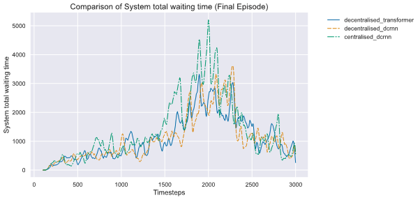
Figure 10: Graph plotting trained models’ performance across 3,000 steps, with total waiting time (seconds) of vehicles per time step.
图 10:绘制了训练模型在 3000 步内的性能,显示了每一步车辆的总等待时间(秒)。
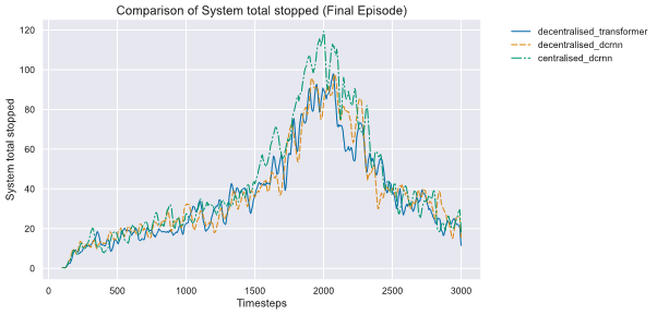
Figure 11: Graph plotting trained models’ performance across 3,000 steps, with total vehicles stopped in traffic per time step.
图 11:绘制了训练模型在 3000 步内的性能,显示了每一步交通中停止的车辆总数。
From the plot, we can observe decentralised control policy has much better performance against centralised control [Figure 10, Figure 11]. And it also indicates that our learned policy can perfectly adapt to the real time traffic (peak vs non-peak).
从图中我们可以观察到,去中心化控制策略相比于中心化控制表现要优越得多[图 10,图 11]。同时,这也表明我们学习到的策略能够完美适应实时交通(高峰与平峰时段)。
Beyond the system level measure, we also try to capture whether there is bottleneck within our system, so we draw the heatmap of agent level metrics to identify it.
除了系统层面的指标,我们还尝试捕捉系统中是否存在瓶颈,因此我们绘制了智能体层面的指标热力图来识别它。
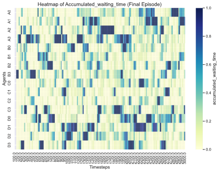
Figure 12: Heatmap of decentralized graph-transformer model indicating normalized waiting time at each traffic signal at each time step.
图 12:去中心化图 Transformer 模型指示的每个时间步每个交通信号点的归一化等待时间热力图。
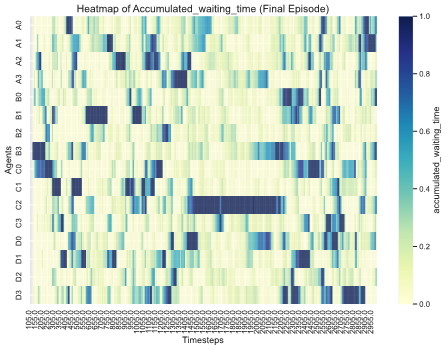
Figure 13: Heatmap of centralized DCRNN model indicating normalized waiting time at each traffic signal at each time step.
图 13:中心化 DCRNN 模型指示的每个时间步每个交通信号点的归一化等待时间热力图。
From the heatmaps, it is evident that the centralized DCRNN model exhibits a clear bottleneck at traffic signal C2 [Figure 12, Figure 13]. This is likely due to the centralized agent needing to explore a vast action space to optimize system-level metrics and maximize the global reward. However, it lacks mechanisms to address agent-level optimization effectively.
从热力图可以看出,集中式 DCRNN 模型在交通信号 C2 处存在明显的瓶颈[图 12,图 13]。这可能是由于集中式代理需要探索庞大的动作空间来优化系统级指标并最大化全局奖励,但它缺乏有效处理代理级优化的机制。
In contrast, decentralized control allows each agent to independently learn policies that enable effective collaboration with neighboring agents while simultaneously optimizing their own rewards. This localized approach makes decentralized control inherently more robust and adaptive to individual traffic signals’ needs.
相比之下,分布式控制允许每个代理独立学习策略,从而能够与相邻代理有效协作,同时优化各自的奖励。这种本地化方法使得分布式控制具有更强的鲁棒性和对单个交通信号需求的适应性。
未来工作
Future work could explore the development of richer graph representations by integrating edge features that encapsulate lane-specific traffic details, such as density, queue length, and flow rate. These enhanced representations could offer a more precise understanding of the traffic system, ultimately leading to improved decision-making in traffic signal control [Figure 14].
未来工作可以探索通过整合包含车道特定交通细节的边特征(如密度、排队长度和流量)来开发更丰富的图表示。这些增强的表示可以提供对交通系统更精确的理解,最终导致交通信号控制中的决策改进[图 14]。
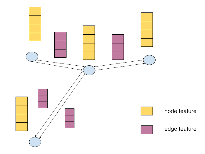
Figure 14: Graph representation with edge features.
图 14:带边特征的图表示。
参考文献
[1] Atwood, J., & Towsley, D. (2016). Diffusion-convolutional neural networks. Advances in neural information processing systems, 29.
[2] Cho, K. (2014). On the properties of neural machine translation: Encoder-decoder approaches. arXiv preprint arXiv:1409.1259.
[3] Chu, T., Wang, J., Codecà, L., & Li, Z. (2019). Multi-agent deep reinforcement learning for large-scale traffic signal control. IEEE transactions on intelligent transportation systems, 21(3), 1086–1095.
[4] Donnat, C., Zitnik, M., Hallac, D., & Leskovec, J. (2018, July). Learning structural node embeddings via diffusion wavelets. In Proceedings of the 24th ACM SIGKDD international conference on knowledge discovery \& data mining (pp. 1320–1329).
[5] Hochreiter, S. (1997). Long Short-term Memory. Neural Computation MIT-Press.
[6] Huang, X., Wu, D., & Boulet, B. (2023). Traffic Signal Control Using Lightweight Transformers: An Offline-to-Online RL Approach. arXiv preprint arXiv:2312.07795.
[7] Li, G., Chen, J., & He, K. (2022). Adaptive Multi-Neighborhood Attention based Transformer for Graph Representation Learning. arXiv preprint arXiv:2211.07970.
[8] Li, Y., Yu, R., Shahabi, C., & Liu, Y. (2017). Diffusion convolutional recurrent neural network: Data-driven traffic forecasting. arXiv preprint arXiv:1707.01926.
[9] Shi, Y., Huang, Z., Feng, S., Zhong, H., Wang, W., & Sun, Y. (2020). Masked label prediction: Unified message passing model for semi-supervised classification. arXiv preprint arXiv:2009.03509.
[10] Staudemeyer, R. C., & Morris, E. R. (2019). Understanding LSTM — a tutorial into long short-term memory recurrent neural networks. arXiv preprint arXiv:1909.09586.
[11] Zhang, Y., Yu, Z., Zhang, J., Wang, L., Luan, T. H., Guo, B., & Yuen, C. (2023). Learning Decentralized Traffic Signal Controllers with Multi-Agent Graph Reinforcement Learning. IEEE Transactions on Mobile Computing.


内容中包含的图片若涉及版权问题,请及时与我们联系删除

评论
沙发等你来抢