
Stanford CS224W: Machine Learning with Graphs
By Tianyang Chen, Tracy Han, Alycia Lee as part of the Stanford CS 224W Final Project

Graph of complex, dynamic system. 复杂动态系统的图。
Graph Neural Networks (GNN) can be used to perform node-, edge-, and graph-level tasks by learning the node embeddings of graphs. However, many graphs are not static. They often evolve over time or when triggered with specific events or conditions, changing the node or edge features or even graph structures. Additionally, due to the nature of network structures, a single change could generate cascading changes to the network. When graphs are highly complex and dynamic, identifying the root cause of the change becomes challenging.
图神经网络(GNN)可以通过学习图的节点嵌入来执行节点级、边级和图级任务。然而,许多图不是静态的。它们通常随着时间的推移或被特定事件或条件触发而演变,改变节点或边特征甚至图结构。此外,由于网络结构的性质,单个变化可能会引发网络的级联变化。当图高度复杂且动态时,识别变化的原因变得具有挑战性。
One real-world example is in software engineering, in which one of the techniques to increase test-ability and achieve separation of concerns in large scale systems is to organize software into independent modules. When connecting multiple software modules together via some communication medium, they collaborate and work to achieve the same goal. For example, open source frameworks such as Apache Airflow(https://airflow.apache.org/) or Robotic Operation Systems(https://www.ros.org/), allow users to organize software into dependent units to form data processing pipelines. This network of software modules could be modeled as a directed cyclic graph: each node represents a module, which consumes input from other modules and produces output for downstream nodes.
一个实际世界的例子是软件工程,其中一种提高可测试性并在大型系统中实现关注点分离的技术是将软件组织成独立的模块。当通过某种通信媒介将多个软件模块连接在一起时,它们会协作并共同实现同一个目标。例如,Apache Airflow 或机器人操作系统等开源框架允许用户将软件组织成依赖单元以形成数据处理管道。这个软件模块的网络可以表示为一个有向循环图:每个节点代表一个模块,它从其他模块消耗输入并为下游节点产生输出。
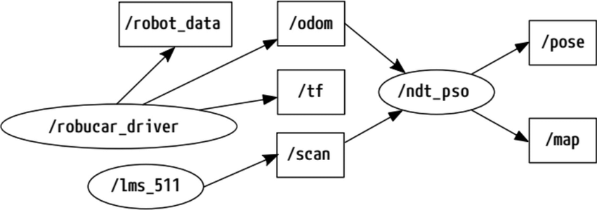
Example ROS Directed Graph Forming A Data Processing Pipeline: researchgate.net
形成数据处理管道的 ROS 有向图:researchgate.net
However, this architecture suffers from the issue of cascading failure, where one node failing could lead to downstream nodes failing in a cascading manner. Failures may manifest in different forms, such as a node receiving invalid input and generating garbage output or becoming completely silent due to a software crash. For complex graphs, troubleshooting becomes difficult when users need to handle a flood of log data or alerts and may require specialized domain knowledge to localize the root cause in an efficient manner. Having a method to predict or identify the root cause when failures occur is therefore essential to maintaining system reliability and minimizing downtime.
然而,这种架构存在级联故障的问题,即一个节点的故障可能导致下游节点以级联方式相继失效。故障可能以不同的形式表现出来,例如节点接收无效输入并生成垃圾输出,或由于软件崩溃而完全沉默。对于复杂的图,当用户需要处理大量的日志数据或警报时,排错会变得困难,并且可能需要专门的领域知识才能以高效的方式定位根本原因。因此,在故障发生时能够预测或识别根本原因对于保持系统可靠性和最小化停机时间至关重要。
Inspired by this real world challenge, we are interested in experimenting with GNN methods to model dynamic systems and perform Root Cause Analysis (RCA) on scenarios modeled after the software engineering example provided.
受到这个现实挑战的启发,我们对使用 GNN 方法对动态系统进行建模,并在类似于所提供的软件工程示例的场景中进行根本原因分析 (RCA) 感兴趣。
Motivations For Creating Our Own Simulator
创建我们自己的模拟器的动机
In our literature review, we found that real-world data that captures such failing scenarios is often proprietary. Most RCA-related publications we came across used proprietary datasets or simulated their own data ([1], [2], [3], [4]), but did not provide simulation code nor sufficient details on how faults were injected. Therefore, we developed a graph executor that allows us to generate graph features and inject faults in a controlled and systematic manner. Given a set of nodes and edges, with each edge representing a publish-subscribe relationship between nodes, the executor generates node features of the graph at each timepoint based on a predefined rule provided by users.
在我们的文献综述中,我们发现能够捕捉此类故障场景的真实世界数据通常是专有的。我们遇到的许多与根本原因分析(RCA)相关的出版物都使用了专有数据集或模拟了自己的数据([1], [2], [3], [4]),但没有提供模拟代码或关于如何注入故障的足够详细信息。因此,我们开发了一个图执行器,它允许我们在受控和系统化的方式下生成图特征并注入故障。给定一组节点和边,其中每条边表示节点之间的发布-订阅关系,执行器根据用户提供的前置规则在每个时间点生成图的节点特征。
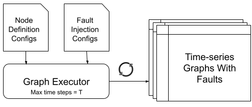
Graph executor configurations and outputs: the graph executor takes node definition configs and fault injection configs as input, then simulates node features of the graph at each timepoint for a maximum number of steps. The output is a time series of node features with fault injected at a timepoint specified by the fault injection config or by the simulation run.
图执行器配置和输出:图执行器将节点定义配置和故障注入配置作为输入,然后模拟每个时间点的图节点特征,最多模拟指定步数。输出是在故障注入配置或模拟运行指定的时间点注入故障的时间序列节点特征。
Users may define connectivity between nodes, as well as node behaviors such as publication, subscription and periodic work with the following Yaml config block:
用户可以定义节点之间的连接关系,以及节点的行为,例如发布、订阅和周期性工作,通过以下 Yaml 配置块:
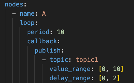
Example yaml config for a node named “A”.
一个名为“A”的节点的示例 Yaml 配置。
A subscribing node may define how it handles incoming messages with the following config block, specifying what to do if message values are out-of-bounds or missing. In the following example, it will further produce wrong messages to affect downstream. It simulates the case where a node receives an invalid input, and responds by sending invalid outputs to other nodes which will affect its neighboring nodes, and propagate to the entire graph over time:
订阅节点可以通过以下配置块定义它如何处理传入的消息,指定如果消息值超出范围或缺失时要做什么。在以下示例中,它将进一步产生错误消息以影响下游。它模拟了节点接收无效输入,并通过向其他节点发送无效输出来响应,这将影响其相邻节点,并随着时间的推移在整个图中传播的情况:
Example yaml config for a node named “B”.
一个名为“B”的节点的示例 Yaml 配置。
Our executor has a rich set of config language that includes delaying/dropping periodic callback, delaying/dropping receipt of new messages and even crashing the node. The following picture shows how nodes are connected via topics specified by the config.
我们的执行器具有丰富的配置语言,包括延迟/丢弃周期性回调、延迟/丢弃接收新消息,甚至崩溃节点。下面的图片显示了节点如何通过配置中指定的主题连接。
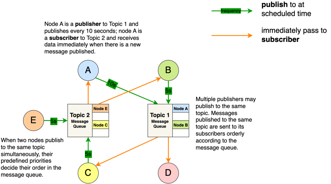
An Example Of Graph Configurations In the Context of Pub-Sub Framework
公共订阅框架上下文中的图配置示例
The configuration of injected faults look like the following:
注入故障的配置如下:
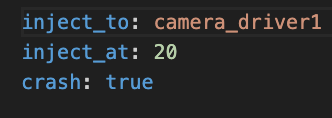
An Example Fault Injection Config That Crashes A Camera Node
一个导致相机节点崩溃的故障注入配置示例
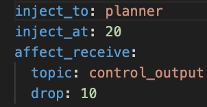
An Example Fault Injection Config That Drops Message Received From A Topic
一个示例故障注入配置,该配置会丢弃从主题接收到的消息
When fault injection configs are provided, our graph executor will perturb the node specified and perform the associated action. Users should expect to see how a dynamic graph system respond to the injected fault immediately. To aid configuration trouble shooting, a complete graph event trace can be inspected.
当提供故障注入配置时,我们的图执行器将扰动指定的节点并执行相关操作。用户应该立即看到动态图系统如何响应注入的故障。为了帮助配置故障排除,可以检查完整的图事件跟踪。
An Example Graph Even Trace For Nodes In the Graph
图中节点的示例图事件跟踪
The task of our GNN methods is to process a time-series of graphs for a system, and determine at which time-point, failure — if it occurs — does occur (graph classification) and identify the node at fault (node classification). This pipeline is illustrated below.
我们 GNN 方法的任务是处理系统的图时间序列,并在时间点确定(如果发生)故障(图分类)并识别故障节点(节点分类)。此流程如下图所示。
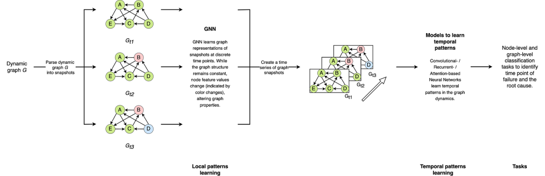
GNN modeling pipeline showing how dynamic graphs are fed through the model, and local and temporal patterns are learned.
GNN 建模流程,展示了动态图如何输入模型,以及如何学习局部和时间模式。
Using a graph executor simulator allows us to generate a vast amount of time-series graph data, and benchmark our model architecture on graphs with different scale or connectivity. For example, we can train a GCN on a graph that resembles autonomous vehicle systems, say with 200 nodes and 1000 edges, and see if such a model would perform well for another graph that mimics online e-commerce systems with say 50 nodes with 200 edges. The training data could be generated by a collection of predefined fault injection actions. Users should be able to configure our simulator to drop any messages published from a node and observe cascading effects of that fault. Furthermore, the simulator also allows a certain amount of randomness in node configuration, enabling us to model real world behavior such as information passing delay between software nodes, or human errors (bugs or non-conformity in code) that can cause nodes to misbehave. To increase the diversity of our training data, our simulator should also allow users to inject multiple faults at different nodes at different times. At the end of this project, we aim to open-source our configuration-based graph executor simulator for the broader research community, to address the aforementioned synthetic data problem from various literature.
使用图执行器模拟器使我们能够生成大量的时间序列图数据,并在具有不同规模或连接性的图上基准测试我们的模型架构。例如,我们可以在一个类似于自动驾驶汽车系统的图(比如有 200 个节点和 1000 条边)上训练一个 GCN,看看这样的模型是否也能很好地处理另一个模拟在线电子商务系统的图(比如有 50 个节点和 200 条边)。训练数据可以通过一系列预定义的故障注入操作生成。用户应该能够配置我们的模拟器来丢弃节点发布的任何消息,并观察该故障的级联效应。此外,模拟器还允许节点配置中存在一定程度的随机性,使我们能够模拟现实世界的行为,例如软件节点之间的信息传递延迟,或可能导致节点行为异常的人为错误(代码中的错误或不一致)。为了增加我们训练数据的多样性,我们的模拟器还应该允许用户在不同的时间在不同的节点注入多个故障。 在此项目结束时,我们旨在向更广泛的研究社区开源我们的基于配置的图执行器模拟器,以解决上述合成数据问题。
With our graph executor, we created a graph configuration that approximates modern autonomous vehicle software architecture (with reasonably similar topology), and injected different faults to the graph at different times to collect a large amount of graph data. The executor is capable of generating visualizations for users to understand dynamic graph systems. Blue nodes denote nominal nodes while red nodes denote faulted nodes.
通过我们的图执行器,我们创建了一个图配置,该配置近似于现代自动驾驶汽车软件架构(拓扑结构相当相似),并在不同时间向图中注入不同的故障,以收集大量图数据。执行器能够为用户提供动态图系统的可视化,蓝色节点表示正常节点,红色节点表示故障节点。
For example, autonomous vehicle software stack typically include sensor, mapping, perception, motion planner and control subsystems. When we crash a camera sensor module, which is the lowest layer in the software stack, the fault will first cause a cluster of mapping and perception nodes to fail, and then affect the motion planning system, eventually causing the vehicle control to fail:
例如,自动驾驶汽车软件堆栈通常包括传感器、地图、感知、运动规划和控制系统等子系统。当我们崩溃相机传感器模块时,这是软件堆栈的最低层,故障将首先导致映射和感知节点集群失效,然后影响运动规划系统,最终导致车辆控制失效:
Crashing A Camera Node Leads To Cascading Failures
崩溃相机节点导致级联故障
Similarly, when we stall the GPS driver, the mapping and localization system would start to fail first, causing the same cascading failure in perception, motion planning and control.
类似地,当我们停止 GPS 驱动程序时,地图和定位系统会首先开始失效,导致感知、运动规划和控制系统中的级联失效。

Stalling A GPS Node Leads To Cascading Failures
停止 GPS 节点会导致级联失效
On the other hand, users are able to inject a less severe fault in the middle of the software stack, which only causes failures to a single subsystem (mapping) without affecting downstream subsystems, due to the fact that they are somewhat resilient towards this injected fault. In this example, the failure propagation pattern can be characterized as local:
另一方面,用户能够在软件堆栈的中间注入一个较轻微的故障,这只会导致单个子系统(地图)的失效,而不会影响下游子系统,因为它们对这个注入的故障有一定的弹性。在这个例子中,故障传播模式可以描述为局部:

Stalling Map Node Processing Leads To Locally Confined Faults To Mapping Subsystem
停止地图节点处理会导致映射子系统局部受限的故障
As you can see, some faults show periodic behavior, as nodes typically perform work periodically. Depending on the severity and location of where a fault is injected, it takes some time for faults to spread and the pattern is highly unpredictable by humans without domain expert knowledge. This simulator proves to be crucial to study the behavior of dynamic graph systems. Our repo contains a diverse list of faults that were injected into our example autonomous driving graph, which were used to generate training datasets. To further increase the diversity of our datasets, the graph executor is able to perform a sweep of all available faults, and inject them at different times. A dynamic graph system may respond differently depending on when a Fault is injected. Fault injection simulation at this scale is usually hard to achieve in the real world, but it is extremely feasible with our graph executor as long as users can provide corresponding configurations.
正如您所见,某些故障表现出周期性行为,因为节点通常会周期性地执行工作。根据故障注入的严重程度和位置,故障传播需要一定时间,并且对于没有领域专家知识的普通人来说,这种模式是高度不可预测的。这个模拟器被证明对于研究动态图系统的行为至关重要。我们的代码库包含了一系列注入到我们的自动驾驶示例图中的故障,这些故障被用来生成训练数据集。为了进一步提高数据集的多样性,图执行器能够对所有可用的故障进行扫描,并在不同的时间注入它们。动态图系统可能根据故障注入的时间不同而做出不同的响应。在如此规模的故障注入模拟通常在现实世界中很难实现,但只要用户能够提供相应的配置,使用我们的图执行器就非常可行。
数据集
To construct a dataset for model training, we processed the output of a simulation run from the graph executor using node and fault configs that specify the graph visualized in the gifs above. The simulation output consists of a time series of node features, the graph structure (i.e. edges connecting nodes), and fault labels (the node at fault and the timestamp of the fault). Each torch_geometric.data object in the dataset represents a “snapshot”, which is an instance of G with its corresponding node features and labels at a given t_i. These snapshots were then fed in chronological order, from time t_1 to t_n to help the model distinguish between healthy and failure states of the system, and mimic how such a RCA tool would function at inference time in real life on a stream of graph datasets for real-time classification.
为了构建用于模型训练的数据集,我们处理了图执行器模拟运行的输出,使用了指定上述 gif 中显示的图的节点和故障配置。模拟输出包括节点特征的时序数据、图结构(即连接节点的边)以及故障标签(故障节点和故障时间戳)。数据集中的每个 torch_geometric.data 对象代表一个“快照”,即给定 t_i 时刻的图 G 及其对应的节点特征和标签。这些快照按时间顺序从时间 t_1 到 t_n 输入,以帮助模型区分系统的健康和故障状态,并模拟真实生活中推理时此类 RCA 工具在实时分类流式图数据集上的功能。
For each torch_geometric.data object, the node features are of dimension num nodes x num features. There are 9 features for each node:
对于每个 torch_geometric.data 对象,节点特征的维度为 num nodes x num features 。每个节点有 9 个特征:
Number of subscriptions 订阅数量
Number of publications 发布数量
Loop period 循环周期
Last event timestamp 最后事件时间戳
Last event type 最后事件类型
Callback type 回调类型
Loop count 循环计数
Received message total count 接收消息总数
Published message count 发布消息数
The node labels are of dimension num nodesx1 where every node is labeled as 0 if healthy, else, 1 if the node is a root cause node. We persist this node label of 1 for the root cause node in snapshots that occur after the timestamp of fault.
节点标签的维度为 num nodes x 1 ,其中每个节点被标记为 0 表示健康,否则,如果节点是根本原因节点,则标记为 1。我们在故障时间戳之后发生的快照中持久化根本原因节点的标签 1。
建模与分析
Using our graph generator, we simulated a graph dataset based on an autonomous vehicle as the model dynamic system. Our goal is to apply GNNs to classify the root cause node (labeled 1) in the above dynamic network system. The simulated dynamic graph dataset has four main traits: firstly, the dataset has both local and temporal patterns as faults tend to spread with periodic pattern; secondly, the graphs are directed and heterogeneous; thirdly, the dataset is highly imbalanced due to anomaly events being rare. In this project, we treated the graphs as homogeneous for simplicity and experimented with three types of graph convolutional layers: GCN, GraphSAGE, and GAT.
使用我们的图生成器,我们基于自动驾驶车辆作为模型动态系统模拟了一个图数据集。我们的目标是将 GNN 应用于分类上述动态网络系统中的根本原因节点(标记为 1)。模拟的动态图数据集具有四个主要特征:首先,数据集具有局部和时序模式,因为故障往往会以周期性模式传播;其次,图是定向和异构的;第三,由于异常事件罕见,数据集高度不平衡。在这个项目中,我们将图视为同构的,以简化问题,并实验了三种类型的图卷积层:GCN、GraphSAGE 和 GAT。
Directed graph learning 定向图学习
In our simulated system, the communication between nodes is directed, therefore the edge src->dst should be treated differently from dst->src. We customized three directed convolutional layers: DirectedGCNConv,DirectedSAGEConv , DirectedGATConv. To keep it a fair comparison across convolutional types, the directed layer adopts the same mechanism to learn directional difference by applying separate weight matrices for src->dst vs. dst->src.
在我们的模拟系统中,节点之间的通信是定向的,因此边 src->dst 应该与边 dst->src 不同。我们定制了三种定向卷积层: DirectedGCNConv 、 DirectedSAGEConv 、 DirectedGATConv 。为了在卷积类型之间保持公平的比较,定向层通过为 src->dst 与 dst->src 应用不同的权重矩阵来学习定向差异。
DirectedGCNConv(
   (src_to_dst_conv): GCNConv(9, 18, aggr=mean)
   (dst_to_src_conv): GCNConv(9, 18, aggr=mean)
 )
 DirectedSAGEConv(
   (src_to_dst_conv): SAGEConv(9, 18, aggr=mean)
   (dst_to_src_conv): SAGEConv(9, 18, aggr=mean)
   (lin_self): Linear(in_features=9, out_features=18, bias=True)
 )
 DirectedGATConv(
   (src_to_dst_conv): GATConv(9, 18, heads=18)
   (dst_to_src_conv): GATConv(9, 18, heads=18)
 )
Rare event detection 稀有事件检测
Anomoly events are rare in the real world, and our simulation aligns with this phenomenon. On average, the number of graphs that contain an anomaly node vs. normal nodes is about 1:4, and by counts at the node level, anomaly node abundance vs. normal nodes is about 1:100. Moreover, the graph contains only normal nodes in timestamped snapshots until the fault injection happens, which poses an additional challenge in balancing classes in the time series dataset as the model will not be exposed to anomaly samples at the beginning of each simulation episode.
在现实世界中,异常事件是罕见的,而我们的模拟与此现象一致。平均而言,包含异常节点的图与正常节点的图的比例约为 1:4,而在节点级别上,异常节点与正常节点的数量比约为 1:100。此外,在故障注入发生之前的每个时间戳快照中,图中只包含正常节点,这给平衡时间序列数据集中的类别带来额外的挑战,因为模型在每次模拟周期的开始时都不会接触到异常样本。
Additionally, from a practical perspective in real world applications, the risk of missing an anomaly detection is likely higher than having oversensitive detection that sometimes misclassifies normal events. Therefore, we designed a more aggressive training strategy that prioritizes rare event detection over global accuracies and applied this strategy to all models for comparative analysis. The strategy has three main components: weighted loss computation by classes, focal loss back-propagation, and early stopping supervised by macro recall scores.
此外,从现实世界应用的实际角度来看,错过异常检测的风险可能高于有时会错误分类正常事件的过度敏感检测。因此,我们设计了一种更积极的训练策略,该策略优先考虑稀有事件检测而不是全局精度,并将此策略应用于所有模型以进行比较分析。该策略有三个主要组成部分:按类别计算加权损失、焦点损失反向传播和由宏观召回分数监督的早停。
Weighted loss computation by classes
按类别计算加权损失
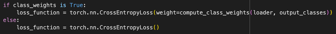
class_weights is computed as:
class0_weight = total # of graphs / # of graphs containing class0
class1_weight = # of graphs containing class1:class0 ratio * total # of graphs / # of graphs containing class1

# Compute class weights example:
Total number of graphs: 9367, Presence of class 0: 9367, Presence of class 1: 2368
tensor([ 1.0000, 15.6472])
This weighted loss computation penalizes the model more when it misclassifies an anomaly event.
这种加权损失计算会在模型错误分类异常事件时对其进行更大的惩罚。
Customized focal loss back-propagation
自定义焦点损失反向传播
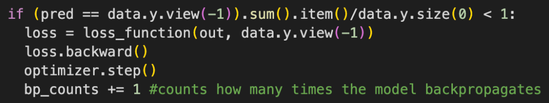
By conditioning the back-propagation on whether the model’s predictions are perfect, this method ensures that the model only updates its parameters when there are errors. This approach can also potentially lead to faster convergence by avoiding wasteful updates when the model is already performing optimally on a given batch. It forces the model to focus its learning capacity on more challenging or wrongly classified examples.
通过在反向传播时根据模型的预测是否完美来调整,这种方法确保模型只在存在错误时更新其参数。这种方法还可以通过避免在模型对某一批次已经表现最优时进行无用更新,从而潜在地加快收敛速度。它迫使模型将其学习能力集中在更具挑战性或错误分类的示例上。
Macro recall score supervised early stopping
宏召回分数监督早期停止
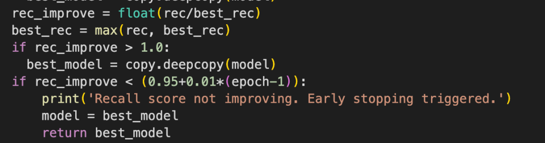
This method prioritizes rare event detection over global accuracies by stopping the model training early when the macro recall score is not improving effectively or efficiently. Since the recall score measures the model’s ability to find all relevant instances of a class, and the macro recall score is calculated unbiasedly by the abundance of a specific class, this forces the model to stop depending on its performance on anomaly detection rather than optimizing weighted accuracies globally across all classes. Furthermore, the mechanism expects the model to perform better as it trains for more epochs. The threshold that triggers early stopping increases over epochs by requiring the model to perform >= (0.95+0.01*(epoch-1))of its best performance. This ensures the model stops training when the learning is not efficient.
这种方法通过在宏观召回率分数没有有效或高效提升时提前停止模型训练,优先检测稀有事件,而不是全局精度。由于召回率分数衡量模型找到某个类别所有相关实例的能力,而宏观召回率分数通过类别丰富度进行无偏计算,这迫使模型根据其在异常检测方面的表现来停止训练,而不是全局优化所有类别的加权精度。此外,该机制预期随着训练进行更多轮次,模型表现会更好。触发提前停止的阈值会随着轮次增加而提高,要求模型达到其最佳表现中的 >= (0.95+0.01*(epoch-1)) 。这确保了当学习效率不高时模型会停止训练。
Spatial and Spatiotemporal modeling
空间和时空建模
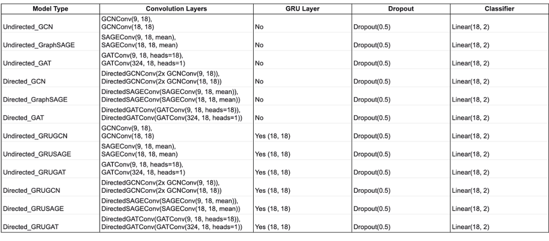
All models apply two convolutional layers followed by a linear layer for classification. Both spatial and spatiotemporal models use the sigmoid activation function before each convolutional layer and apply one dropout layer between two convolutional layers. Additionally, all spatiotemporal models apply one GRU layer post-convolution to track the hidden states of each node. The diagram below shows the architectures of spatial and spatiotemporal models.
所有模型都应用两个卷积层,然后接一个线性层进行分类。空间模型和时空模型在每个卷积层之前都使用 sigmoid 激活函数,并且在两个卷积层之间应用一个 dropout 层。此外,所有时空模型在卷积层之后应用一个 GRU 层来跟踪每个节点的隐藏状态。下图显示了空间和时空模型的结构。
模型结构
结果
实验设置
The combination of [GCNConv, SAGEConv, GATConv], [undirected, directed], and [-GRU, +GRU] yields a total of 12 candidate models. With a fixed learning rate = 0.001 and weight decay rate = 5e-4, we trained each of the model candidates on one instance of a specific type of fault, and evaluated the trained model on three questions:
[GCNConv, SAGEConv, GATConv] 、 [undirected, directed] 和 [-GRU, +GRU] 的组合产生了 12 个候选模型。在固定的 learning rate = 0.001 和 weight decay rate = 5e-4 下,我们针对特定类型的故障的每个模型候选进行了训练,并在三个问题上评估了训练好的模型:
1. How does the model perform on its training dataset?
   Example dataset used in experiments:
   crash_camera_driver1, 1 instance, Total number of graphs: 8877, Presence of class 0: 8877, Presence of class 1: 2048

2. How does the model perform on a different instance of the same type of fault?
   Example dataset used in experiments:
   crash_camera_driver1, 1 instance (different from training instance), Total number of graphs: 8843, Presence of class 0: 8843, Presence of class 1: 2048

3. How does the model perform on an instance from a different type of fault?
   Example dataset used in experiments:
   crash_tracker, 1 instance,Total number of graphs: 8914, Presence of class 0: 8914, Presence of class 1: 1988
For spatial models, since the chronological order of time points is not used, the data loader shuffles the dataset; for spatiotemporal models, the data loader does not shuffle and passes graphs to the model in chronological order.
对于空间模型,由于时间点的时序顺序不被使用,数据加载器会打乱数据集;对于时空模型,数据加载器不会打乱,而是按时间顺序将图传递给模型。
Experiment 1: training and evaluating models on the standard simulations
实验 1:在标准模拟上进行模型训练和评估
In this first experiment, we trained and evaluated our models on the standard dataset. The dataset includes a total of 200 instances. Each instance is generated by simulating one of the following faults injected at a random timestamp: crash_camera_driver1, crash_tracker, drop_raw_camera1_publish, drop_raw_camera1_receive, mutate_raw_camera1_publish. During every instance, the simulation creates between 8,000–10,000 graphs, representing discrete snapshots of the dynamic system at a specific timestamp. Each graph has 29 nodes with 9 features per node, 41 directed edges, and 29 binary node-level labels where 0 indicates a healthy functioning node and 1 indicates a mutated faulty node. The dynamic system remains static structurally over time, i.e., graph snapshots are structurally identical during an instance, but feature values are dynamic due to autonomous node behaviors.
在第一个实验中,我们在标准数据集上训练和评估了我们的模型。该数据集总共包含 200 个实例。每个实例是通过在随机时间戳处模拟以下故障之一生成的:crash_camera_driver1 、crash_tracker 、 drop_raw_camera1_publish 、drop_raw_camera1_receive 、 mutate_raw_camera1_publish 。在每个实例中,模拟会创建 8,000–10,000 个图,代表动态系统在特定时间戳的离散快照。每个图有 29 个节点,每个节点有 9 个特征,41 条有向边,以及 29 个二进制节点级标签,其中 0 表示节点正常工作,1 表示节点发生故障。动态系统在结构上随时间保持静态,即在一个实例中,图快照在结构上是相同的,但由于自主节点行为,特征值是动态的。
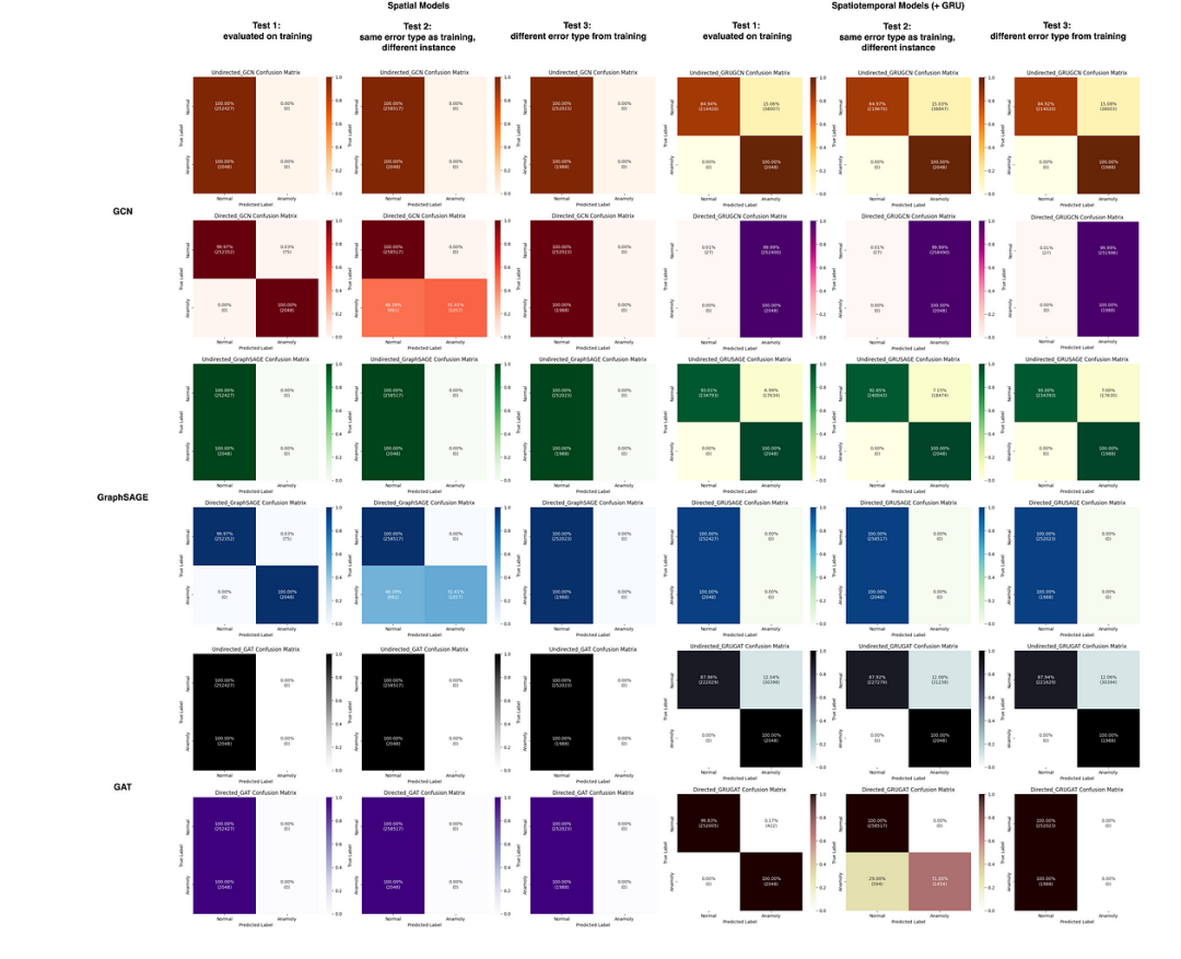
The diagram below shows the confusion matrices generated by each model when tested.
下面的图表显示了每个模型在测试时生成的混淆矩阵。
Access these confusion matrices, training and testing logs, and code of this experiment here.
您可以在这里访问这些混淆矩阵、训练和测试日志以及此实验的代码。
===== Quick Stats =====
Precision: Measures the accuracy of positive predictions.
Recall: Measures the model’s ability to find all relevant instances of each class.
F1-Score: The harmonic mean of precision and recall, which balances the two metrics.
Support: The number of true instances for each class.
Macro Average: Takes the average of each metric without considering the class support, providing an unweighted view.
Weighted Average: Takes the average of each metric, weighted by the number of instances in each class.
Overall, in spatial models, applying directed convolutional layers yields higher performance than applying undirected convolutional layers. Directed spatial GCN and GraphSAGE models demonstrate high performance when evaluated on their training instance (test 1), perform worse on the same error type but different instance (test 2), and collapse on the unseen error type (test 3), suggesting overfitting and poor generalizability. In spatiotemporal models, however, undirected convolutional layers yield better results. Undirected spatiotemporal GCN, GraphSAGE, and GAT perform similarly impressive across all tests (100% accuracy at identifying anomaly), suggesting that temporal learning enhances the model’s generalizability and is potentially more logical. Recall that the graph system remains structurally static at any time and in any situation, therefore, these observation indicates that the type of fault injected uniquely and effectively impacts the network and that the models are learning fault-specific knowledge rather than relying on systematic common sense.
总的来说,在空间模型中,应用有向卷积层比应用无向卷积层能获得更高的性能。有向空间 GCN 和 GraphSAGE 模型在评估其训练实例(测试 1)时表现出高性能,在相同错误类型但不同实例(测试 2)上表现较差,并且在未出现的错误类型(测试 3)上崩溃,这表明过拟合和泛化能力差。然而,在时空模型中,无向卷积层能获得更好的结果。无向时空 GCN、GraphSAGE 和 GAT 在所有测试中都表现出类似的高性能(在识别异常方面达到 100%的准确率),这表明时间学习增强了模型的泛化能力,并且可能更符合逻辑。回想一下,图系统在任何时间和情况下都保持结构上的静态,因此,这些观察结果表明注入的故障类型独特且有效地影响了网络,并且模型在学习特定于故障的知识,而不是依赖于系统的常识
Among all candidates, 6 out of 12 models achieved a 100% (2048/2048) anomaly detection rate when evaluated on the training instance (recall score for class 1 = 1; no misclassification of class 1). The 6 models are: Directed GCN (spatial), Directed GraphSAGE (spatial), Undirected GRUGCN (spatiotemporal), Undirected GRUGAT (spatiotemporal), Undirected and Directed GRUGAT (spatiotemporal).
在所有候选模型中,有 6 个模型在训练实例上的评估中达到了 100%(2048/2048)的异常检测率(类别 1 的召回得分为 1;类别 1 没有误分类)。这 6 个模型是:有向 GCN(空间)、有向图 SAGE(空间)、无向 GRUGCN(时空)、无向 GRUGAT(时空)、无向和有向 GRUGAT(时空)。
In summary, spatiotemporal models outperform spatial models due to their generalizability across test scenarios. The experiment results align with the spatiotemporal nature of our dataset.
总之,时空模型优于空间模型,因为它们在测试场景中的泛化能力更强。实验结果与数据集的时空特性相符。
Additional food for thought:
一些额外的思考:
Local communication patterns (captured by spatial modeling) of the dynamic system might be more informative of node behavioral health in some error types than the temporal history (captured in temporal learning) of an individual node’s behaviors, and vice versa.
动态系统的局部通信模式(由空间建模捕获)在某些错误类型中可能比个体节点行为的历史(由时间学习捕获)更能反映节点的行为健康状况,反之亦然。
Global fault propagation could exhibit a periodic pattern where clusters of nodes oscillate between nominal and failing, which could require the model to remember a long history before it becomes useful.
全局故障传播可能表现出周期性模式,其中节点集群在正常和故障状态之间振荡,这可能需要模型记住较长的历史记录才能变得有用。
Applying GRU post-convolutions may not be the best practice, and it raises the question of whether applying GRU before convolutions is better than applying GRU post-convolutions.
应用 GRU 后卷积可能不是最佳实践,并且它提出了一个问题,即应用 GRU 在卷积之前是否比应用 GRU 后卷积更好。
Adjusting hyperparameters such as hidden dimensions, dropouts, and learning rates and applying batch normalization across time points may be helpful in reducing overfitting and pushing the models to learn more effectively.
调整隐藏维度、dropout 和学习率等超参数,并在时间点应用批量归一化可能有助于减少过拟合,并推动模型更有效地学习。
Experiment 2: training and evaluating models on more complex simulations
实验 2:在更复杂的模拟上训练和评估模型
Using the same experimental setup as before, we trained and evaluated these models using a dataset that extends the previous graph and makes it more complex by adding more nodes (for a total of 46 nodes) and more edge connections between software modules. A visualization of this augmented graph can be observed in the fault visualizations (.gifs) shown in previous sections. The results on test data are shown below, after training the models on data with the fault of camera driver #1 crashing being injected at a random timepoint:
使用与之前相同的实验设置,我们使用一个扩展了先前图并使其更复杂的数据库来训练和评估这些模型,通过添加更多节点(总共 46 个节点)和更多软件模块之间的边连接。可以在之前章节中显示的故障可视化(.gifs)中观察到这个增强图的可视化。在训练模型时注入了相机驱动器#1 崩溃的故障数据,并在测试数据上显示了结果:
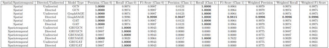
GNN model results on unseen data of the same fault type (crash camera driver #1) as the model was trained on. The highest scores in each column are bolded. Access the Colab notebook of this experiment here.
GNN 模型在未见过数据的相同故障类型(相机驱动器#1 崩溃)上的结果,该模型是在训练数据上训练的。每列中的最高分已加粗。访问此实验的 Colab 笔记本。
Based on these results, we observed that in general, directed models outperform their undirected counterparts, and the spatial models performed better than spatiotemporal models. Of the spatial models, the GCN and GAT models have similar performance, with high precision and recall for class 0, and lower precision but high recall for class 1. This makes sense given that the dataset is inherently imbalanced in that there are more instances of nodes labeled 0 than 1. The directed GraphSAGE model shows the best performance overall, with high precision, recall, and F1-score for both classes.
基于这些结果,我们观察到一般来说,有向模型比无向模型表现更好,而空间模型的表现优于时空模型。在空间模型中,GCN 和 GAT 模型的性能相似,对于类别 0 具有较高的精确率和召回率,而对于类别 1 精确率较低但召回率较高。考虑到数据集在本质上是不平衡的,即标记为 0 的节点实例多于标记为 1 的节点,这是可以理解的。有向 GraphSAGE 模型总体表现最佳,对于两个类别都具有较高的精确率、召回率和 F1 分数。
Of the spatiotemporal models, the GRUGCN and GRUGAT models struggle significantly with class 1 predictions, showing 0 performance in precision, recall, and F1-score. The directed GRUSAGE model shows some improvement in Class 1 predictions but still underperforms compared to spatial models.
在时空模型中,GRUGCN 和 GRUGAT 模型在类别 1 的预测方面表现不佳,精确率、召回率和 F1 分数均为 0。有向 GRUSAGE 模型在类别 1 的预测方面有所改进,但与空间模型相比仍然表现不佳。
We observed that several models had the same scores across the metrics, e.g. undirected and directed GCNs, and undirected GraphSAGE. After ruling out the possibility of a bug in our code, since these models were observed to have different training metrics, we came to the conclusion that the similarity in scores was due to the prediction mechanism we use: after applying a sigmoid layer to obtain predicted scores for classes 0 and 1, the class with the maximum score for each node is the predicted value. Therefore, the final prediction is determined by the relative scores rather than the absolute differences. This approach can lead to identical classification results when the relative rankings of the predicted scores are consistent across different models.
我们观察到几个模型在各项指标上的得分相同,例如无向和有向 GCN,以及无向 GraphSAGE。在排除了代码中存在 bug 的可能性后,由于观察到这些模型具有不同的训练指标,我们得出结论,得分相似性是由于我们使用的预测机制:在应用 sigmoid 层以获得类别 0 和 1 的预测得分后,每个节点的最高得分对应的类别是预测值。因此,最终预测由相对得分决定,而不是绝对差异。当不同模型中预测得分的相对排名一致时,这种方法可能导致相同的分类结果。
总结
We have implemented a graph executor with fault injection capability to allow us to study how dynamic graphs respond to anomaly. Even though the scope of the executor is to approximate pub-sub graphs, with various simplification, it is able to generate and provide use-case agnostic node features, that are fundamental to all pub-sub based systems. In real world use we expect more use-case specific features to improve the Root Cause Analysis Performance. We hope this executor would accelerate future model research.
我们实现了一个具有故障注入功能的图执行器,以允许我们研究动态图如何响应异常。尽管执行器的范围是近似发布-订阅图,通过各种简化,它能够生成并提供与用例无关的节点特征,这些特征是所有基于发布-订阅系统的基本要素。在实际应用中,我们期望更多特定于用例的特征以提高根本原因分析性能。我们希望这个执行器能够加速未来的模型研究。
Based on our experiments, the attention based model performs the best, but to our surprise, temporal based models trail behind. The nature of fault propagation is highly stateful. We therefore recommend future researchers to explore more in this direction. In real world, it is also worth experimenting the model using lossy snapshots where not all feature transitions are available.
基于我们的实验,基于注意力的模型表现最佳,但让我们惊讶的是,基于时间的模型落后于前者。故障传播的性质高度依赖于状态。因此,我们建议未来的研究人员在这个方向上进行更多探索。在现实世界中,也有必要使用有损快照进行实验,其中并非所有特征转换都是可用的。
GitHub 仓库
You can find our GitHub repo for the graph executor simulator here. Please see the README for details on how to run simulations of graph generation. This repo also contains Jupyter notebooks with our modeling pipelines. The infrastructure was setup in a way that allow people to deterministically reproduce the results via Bazel.
您可以在我们的 GitHub 仓库中找到图执行器模拟器的链接(https://github.com/yundddd/graph_generator)。有关如何运行图生成模拟的详细信息,请参阅 README。该仓库还包含包含我们建模流程的 Jupyter 笔记本(https://github.com/yundddd/graph_generator/tree/master/notebooks)。基础设施是按照允许人们通过 Bazel 确定性地重现结果的方式设置的。
参考文献
[1] Ailin Deng and Bryan Hooi. Graph neural network-based anomaly detection in multivariate time series. CoRR, abs/2106.06947, 2021.
[2] Zeyan Li, Junjie Chen, Yihao Chen, Chengyang Luo, Yiwei Zhao, Yongqian Sun, Kaixin Sui, Xiping Wang, Dapeng Liu, Xing Jin, Qi Wang, and Dan Pei. Generic and robust root cause localization for multi-dimensional data in online service systems, 2023.
[3] Dongjie Wang, Zhengzhang Chen, Jingchao Ni, Liang Tong, Zheng Wang, Yanjie Fu, and Haifeng Chen. Hierarchical graph neural networks for causal discovery and root cause localization, 2023.
[4] Chia-Cheng Yen, Wenting Sun, Hakimeh Purmehdi, Won Park, Kunal Rajan Deshmukh, Nishank Thakrar, Omar Nassef, and Adam Jacobs. Graph neural network based root cause analysis using multivariate time-series kpis for wireless networks. In NOMS 2022–2022 IEEE/IFIP Network Operations and Management Symposium, pages 1–7, 2022.


内容中包含的图片若涉及版权问题,请及时与我们联系删除

评论
沙发等你来抢