
Stanford CS224W: Machine Learning with Graphs
Code
https://colab.research.google.com/drive/1DNl8WXc5xt6g1JQWUvZVUMp7GHVDF0P1?usp=sharing
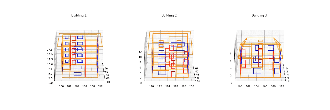
从 Synbuild-3D 数据集重建的 3D 建筑
在这篇博客文章中,我们探索了多种训练图变分自动编码器的方法,用于 3D 建筑线框的生成建模。我们关注了尝试的不同方法,讨论了遇到的困难,并反思了图变分自动编码器在 3D 建筑设计中的应用。
从处理数据集的复杂性到应对训练变分自编码器(VAEs)的复杂性,我们面临了一些影响收敛和性能的挑战。这些问题包括损失函数的不稳定性、学习有意义的潜在表示的困难,以及确保模型与三维建筑数据的多样性和丰富性相一致。
通过记录我们的经验,我们旨在激发讨论并为探索图 VAEs 的研究人员提供潜在的解释,特别是在涉及三维建筑设计应用方面。
动机
我们如何能更好地设计建筑以减少其碳足迹?人工智能(AI)能在自动化这一过程中发挥什么作用?这些问题是推动可持续建筑发展的核心。
建筑物约占全球能源消耗和碳排放的 40%[1]。为应对这一问题,3D 建筑能耗模拟对于改造结构并最小化其环境影响至关重要。然而,创建 3D 建筑模型仍然是一项手动、耗时且昂贵的任务。
这一瓶颈的存在是因为当前的生成算法缺乏自动以图形式创建逼真 3D 建筑模型的能力。
本研究旨在通过探索图生成模型(特别是图变分自编码器[2](图 VAEs))的潜力,以自动化和改进 3D 建筑模型的生成,为更高效和可持续的建筑实践铺平道路。
为什么选择图 VAE?
图变分自编码器(Graph VAEs)被选用于本项目,因为我们的数据集由 3D 建筑线框组成,这些线框可以自然地表示为图。
这种基于图的表示方式与图变分自编码器(Graph VAE)有效学习和生成图结构的能力相契合。图变分自编码器为输入图提供了潜在表示,能够生成新的图样本,这对于自动化 3D 建筑建模至关重要。
图变分自编码器的主要组件包括:一个 Encoder 和一个 Decoder 。
一个Encoder :它将 3D 建筑图映射到潜在空间(一个低维空间)中的 z。
一个Decoder:将 z 映射回高维空间
也有其他选择:
图自动编码器:主要用于嵌入,无法保证潜在空间的分布。它们的生成能力较弱,因此未选择用于本项目。
标准图神经网络是为涉及固定输入图的任务设计的,而不是生成任务。它们本身不提供采样或生成新图实例的机制,而这正是我们项目的核心要求。
数据集和预处理
对于这个项目,我们将使用 SYNBUILD-3D 数据集。
这个数据集包含超过 10 万个 3D 建筑线框。我们选择这个数据集有几个令人信服的理由:
它已经由建筑建模和仿真专家验证过。
包含丰富的几何和语义信息(包括节点/边坐标、门窗/建筑点以及楼层平面图房间细节)
提供全面的建筑内外几何形状,并包含详细的门窗规格。
这里总结了数据集中存在的元素
我们的建筑是一个无向、无权重的图 G = (V, E),其中节点数 N = |V| 因数据集中的每座建筑而异。与原始的 GVAE 论文 [2] 不同,我们不假设每个节点都连接到自身——这对于建筑来说并不现实。
Graphs:
节点:建筑中点的 3D 坐标(窗户点、门点、边缘点),存储在一个 Nx3 的矩阵 X 中。
边:存储在邻接矩阵 A NxN 中的 3D 坐标之间的连接。
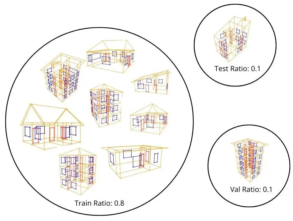
训练集、验证集和测试集比例的示意图。这使读者能够意识到数据集由小图组成,我们是在建筑物之间划分数据集,而不是沿着边进行划分,例如。
我们使用 400 个样本,训练集比例为 0.8,验证集比例为 0.1,测试集比例为 0.1。批处理大小设置为 1。
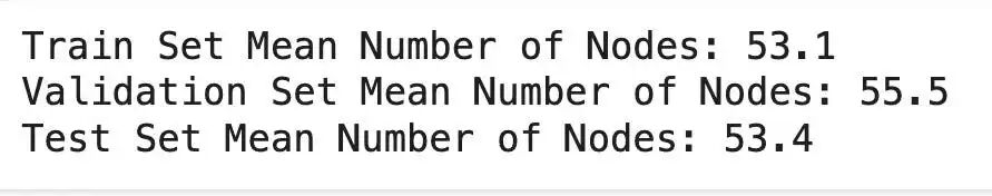
训练集、验证集和测试集中的节点平均数量。
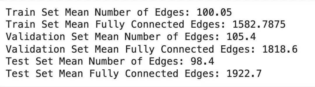
上面的数字是训练集、验证集和测试集中数据集的平均边数。奇数行是如果图是完全连接的,它将拥有的边数。这表明我们数据集中的建筑图不是完全连接的图,因为完全连接图的边数与我们的图之间存在差异。
对于数据集,我们提供了一种有用的数据增强技术( Def rotation )。这种数据增强包括在保持 z 不变的情况下旋转 x-y 轴。
数据增强与增加训练数据的多样性以及提高模型鲁棒性相关。通过在保持 z 不变的情况下旋转 x-y 轴,我们模拟了相同建筑的角度变化。
与其他类型的数据增强技术相反,例如向节点位置添加随机噪声或子图采样。这种方法保留了三维图数据建筑的垂直结构和连通性,并在引入方向变化的同时确保了建筑结构的完整性。
import copy
defrotation(data):
"""Data augmentation by rotating the x and y coordinates while keeping z constant."""
    augmented_data = []  # Initialize empty list for augmented data

for sample in data:
        augmented_sample = copy.deepcopy(sample) # copy to avoid modifying directly the data, as agreed with Kevin.
        angle = random.uniform(0, 2 * np.pi)  # Generate one random angle per sample to flip the x,y axis while keeping z constant

# Create rotation matrix
        rotation_matrix = np.array([
            [np.cos(angle), -np.sin(angle), 0],
            [np.sin(angle), np.cos(angle), 0],
            [0, 0, 1]
        ])

# Rotate all point types with the same angle
for key in ['building_points', 'window_points', 'door_points']:
if key in sample:
                points = np.array(sample[key]) # Convert points to numpy array
                rotated_points = points @ rotation_matrix.T #rotate
                augmented_sample[key] = rotated_points.tolist()  # Convert back to list

        augmented_data.append(augmented_sample)
return augmented_data

# Example usage:
augmented_data = rotation(output_list)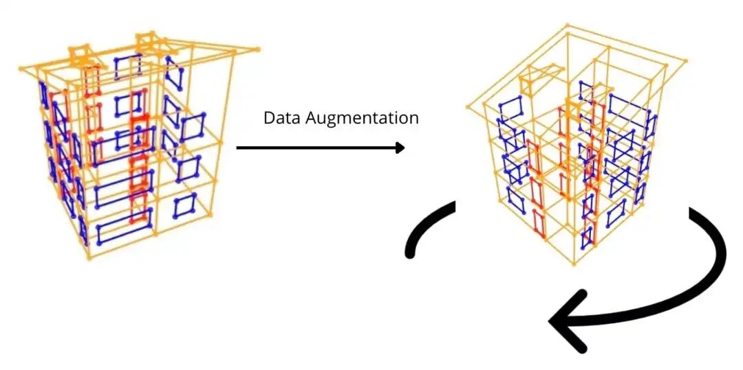
Def Rotation 函数的图示。左侧是数据增强前的 3D 建筑,右侧是数据增强后的建筑。如果我们可视化这栋建筑的 x、y、z 坐标,数据增强会随机地改变 x、y 坐标,而 z 轴保持不变。
变分自编码器:实验#1
我们的目标是学习基于图的建筑表示的生成模型。我们以 Kipf 等人[2]提出的变分图自编码器(VGAE)作为起点。
用 X 表示 N x 3 的节点位置矩阵,用 A 表示图的邻接矩阵。VGAE 由一个编码器 q(z | X, A)和一个解码器 p(A | z)组成,其中 z 是一个 N x H 的矩阵,每一行是一个各向同性高斯分布(H < 3)。
在 VAEs 中,模型通过优化变分下界(ELBO)进行训练,

根据文献[2]中的实现,编码器 q 由一个 2 层 GCN 参数化,该 GCN 输出潜在变量 z 的均值和标准差(也称为重参数化技巧变量)。解码器对条件于潜在变量 z 的邻接矩阵 A 的分布进行建模,表示为

其中σ是 Sigmoid 函数。我们建议读者查阅论文以获取更多细节。
虽然 VGAE 允许我们采样新的邻接结构,但我们希望条件于 z 对节点位置进行建模。为此,我们利用另一个 GCN,该 GCN 以潜在变量 z 为输入,并输出一个 N x 3 的位置矩阵。在训练过程中,我们最小化原始位置 x 与从 z 重建的位置之间的均方误差。
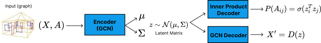
我们提出的用于生成节点位置和边的改进型 VGAE 架构。
遵循论文[2],我们将编码器实现为一个带有 ReLU 激活的图卷积,随后接两个图卷积,一个用于 z 的均值,一个用于对数标准差。
classVGEncoder(torch.nn.Module):
'''Encoder implemented following The Graph Autoencoder paper of Kipf et al. [2]'''
def__init__(self, in_channels=3, out_channels=2):
super().__init__()
        self.conv_init = GCNConv(in_channels, out_channels) # Initial graph convolutional layer to process input features
        self.conv_mu = GCNConv(out_channels, out_channels)  # GCN for mean
        self.conv_logstd = GCNConv(out_channels, out_channels) # GCN for log standard deviation

defforward(self, x, edge_index):
"""
        Forward pass of the VGEncoder.
        """
# Pass input features x through the initial convolution layer
        x = self.conv_init(x, edge_index)

# Compute mean and log_std
        mu = self.conv_mu(x, edge_index) # Compute the mean (mu) of the latent distribution
        log_std = self.conv_logstd(x, edge_index) # Compute the log standard deviation (log_std) of the latent distribution
return mu, log_std  # Return the mean and log standard deviation
如上所述,使用了两个解码器:
p(A|z),它使用 PyG 的 InnerProductDecoder。
一个基于 GCN 的解码器,用于输出位置信息。
EPS = 1e-15

classAVGAE(nn.Module):
'''
    Variational Graph Autoencoder (VGAE) model for graph-based data generation.

    This class defines an autoencoder with a variational approach, consisting of:
    - An encoder to map input data into a latent representation.
    - Decoders to reconstruct both the adjacency matrix and the node positions.

    Here, the Encoder will be VGEncoder from previous cell
    '''
def__init__(self, in_channels=3, hidden_channels=2, out_channels=3):
'''
        Initializes the AVGAE model with
           in_channels (corresponding to the number of input feature (3D coordinates)))
           hidden_channelsl (the lower will be this number the more compressed in the latent space will be our node feature and adjacency matrix)
           out_channels (the number of features to reconstruct)

        '''
super().__init__()
        self.enc = VGEncoder(in_channels=in_channels, out_channels=hidden_channels) # Encoder used to compute latent variables.
        self.adj_dec = InnerProductDecoder() # Decoder for adjacency reconstruction.
        self.pos_dec = GCN(
            in_channels=hidden_channels,
            hidden_channels=hidden_channels,
            out_channels=out_channels,
            num_layers=2,
            act='relu',
        )  # Graph Convolutional Network to decode node positions.

defreparametrize(self, mu: Tensor, logstd: Tensor) -> Tensor:
'''
        Reparameterization trick to sample from a Gaussian distribution.

        Parameters:
        - mu is the mean of the latent distribution.
        - logstd is the Log of the standard deviation of the latent distribution.

        Returns:
        - Sampled latent variable z.
        '''
if self.training:
return mu + torch.randn_like(logstd) * torch.exp(logstd) # Apply reparameterization during training to allow gradient flow.
else:
return mu # Using the mean for inference.

defkl_loss(self, mu: Tensor, logstd: Tensor) -> Tensor:
'''Computes the Kullback-Leibler (KL) divergence loss.'''
return -0.5 * torch.mean(
            torch.sum(1 + 2 * logstd - mu**2 - logstd.exp()**2, dim=1)
        )

defadj_recon_loss(self, z: Tensor, pos_edge_index: Tensor,
                       neg_edge_index: Tensor = None) -> Tensor:
'''Computes the reconstruction loss for the adjacency matrix.'''
# Loss for predicting positive edges.
        pos_loss = -torch.log(self.adj_dec(z, pos_edge_index, sigmoid=True) + EPS).mean()

if neg_edge_index isNone:
            neg_edge_index = negative_sampling(pos_edge_index, z.size(0))
        neg_loss = -torch.log(1 - self.adj_dec(z, neg_edge_index, sigmoid=True) + EPS).mean() # Loss for predicting negative edges.

return pos_loss + neg_loss

defpos_recon_loss(self, x: Tensor, edge_index: Tensor, z: Tensor) -> Tensor:
''' Computes the reconstruction loss for the node positions.'''
        out = self.pos_dec(z, edge_index) # Decode latent z into node positions.
return F.mse_loss(x, out) #MSE (Mean Squared Error) loss for the positions.

defforward(self, x: Tensor, edge_index: Tensor):
'''Forward pass of the AVGAE model.'''
        mu, logstd = self.enc(x, edge_index) # Encode the input into latent variables.
        z = self.reparametrize(mu, logstd)
return (self.pos_recon_loss(x, edge_index, z), # Position reconstruction loss.
                self.adj_recon_loss(z, edge_index),  # Adjacency reconstruction loss.
                self.kl_loss(mu, logstd)) # KL divergence loss.
损失函数包含三个项:
一个用于位置信息的重构误差项(均方误差),鼓励重建的位置接近原始位置。
InnerProductDecoder 预测的邻接矩阵的边概率的负对数似然(NLL),最大化图中存在的边的似然性。
近似后验 q(z|A,X) 与标准正态先验 p(z) 之间的 KL 散度,这鼓励了编码器产生的分布
我们为什么要修改解码器?
由于 3D 点不能是随机的,解码器以及文档中的 InnerProductDecoder 只能解码邻接矩阵,因此我们必须添加一个 3D 位置解码器(一个图卷积网络)。这样,图变分自编码器现在能够解码边概率和位置。
训练
我们使用 1 的批处理大小训练了 200 个 epoch。在整个实验过程中,我们追踪了 KL 损失、边损失、位置损失以及总损失,总损失是位置损失和边损失的组合。
实验#1 的结果
实验#1 是本文中讨论的实现。
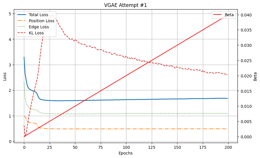
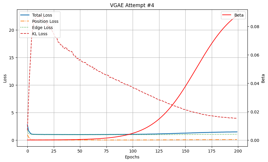
实验#1 的总损失(位置损失+边损失)、位置损失、边损失和 KL 损失。Beta 是 KL 损失的权重,我们使用调度器逐步增加 KL 损失的权重,在 200 个 epoch 时达到 0.04。
我们的第一次 VGAE 训练是在我们数据集的 240 个图子集上进行的,共进行了 200 个 epoch。从图中可以看出,两个重建损失先下降然后稳定。KL 损失最初会爆炸,但随着 KL 权重 beta 的增加,它会缓慢(并且可预测地)下降。
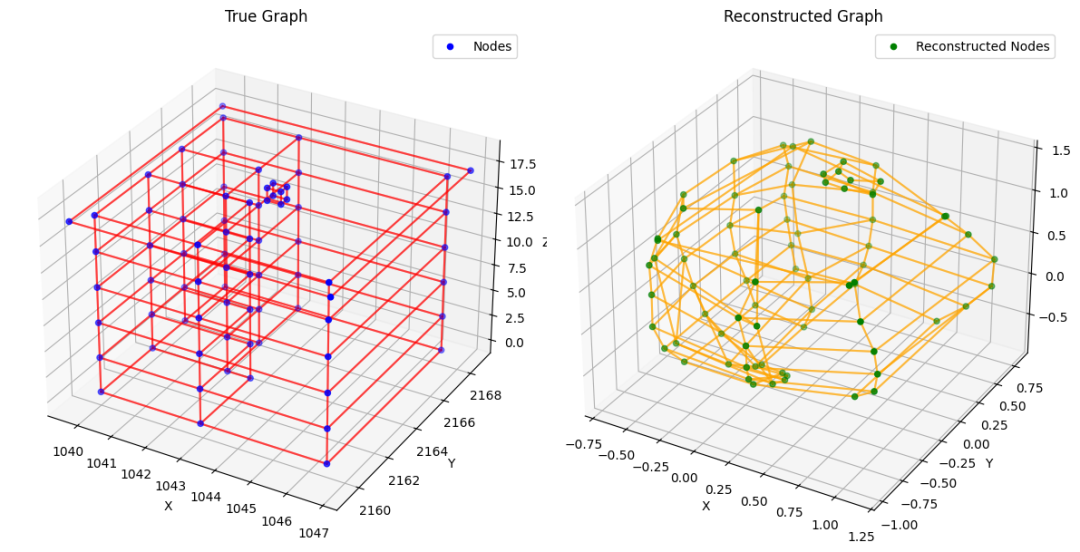
观察数据集中的一个重建示例,会讲述一个不同的故事:
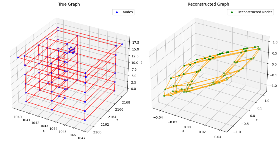
验证样本实验#1
看起来模型缺乏足够的容量来准确地重建我们的图。一个直观的理解可能是,当前的参数数量太低,无法把握 3D 图数据集的复杂性。确实,每个图节点代表 3D 坐标,这本质上编码了复杂的空间关系。
VGAE 实验#2:增加更多层
我们将通过两种方式来缓解上述问题。首先,我们将 VGEncoder 进行泛化,将初始的图卷积替换为多层 GCN。我们将编码器和解码器中的 GCN 层数设置为 4。
其次,我们将编码器 GCN 的隐藏维度从 2 增加到 16,然后再将隐藏维度压缩回 2。我们预计这种调整将使模型能够捕捉数据中更复杂的模式,同时仍然强制执行紧凑的潜在空间( out_channels=2 ),以实现高效的编码。
import torch
import torch.nn as nn
import torch.nn.functional as F
from torch import Tensor
from torch_geometric.nn import GCNConv, InnerProductDecoder
from torch_geometric.utils import negative_sampling

# VGEncoder as previously defined:
classVGEncoder(nn.Module):
'''The encoder maps input graph data (node features and edges) to latent space representations.
    It uses multiple GCN layers to compute the mean and log standard deviation for the latent variables.'''

def__init__(self, in_channels=3, out_channels=2, hidden_channels=16, num_layers=2):
super().__init__()
        self.convs = nn.ModuleList()

# Initial GCN layer
        self.convs.append(GCNConv(in_channels, hidden_channels))
# Add intermediate GCN layers
for _ inrange(num_layers - 2):
            self.convs.append(GCNConv(hidden_channels, hidden_channels))
# Final GCN layer
if num_layers > 1:
            self.convs.append(GCNConv(hidden_channels, out_channels))
else:
            self.convs[0] = GCNConv(in_channels, out_channels)

# Separate layers for computing mean and log standard deviation
        self.conv_mu = GCNConv(out_channels, out_channels)
        self.conv_logstd = GCNConv(out_channels, out_channels)

defforward(self, x, edge_index):
'''Forward pass through the encoder.'''
for i, conv inenumerate(self.convs):
            x = conv(x, edge_index)
if i < len(self.convs) - 1: # Apply activation except for the final layer
                x = F.relu(x)

# Compute mean and log standard deviation
        mu = self.conv_mu(x, edge_index)
        log_std = self.conv_logstd(x, edge_index)
return mu, log_std

EPS = 1e-15

# AVGAE with multi-layer GCN as decoder
classAVGAE(nn.Module):
def__init__(self, in_channels=3, hidden_channels=2, out_channels=3, num_dec_layers=4):
super().__init__()

        self.enc = VGEncoder(in_channels=in_channels, out_channels=hidden_channels)

        self.adj_dec = InnerProductDecoder() # Decoder for adjacency reconstruction.

        self.pos_dec = GCN(
            in_channels=hidden_channels,
            hidden_channels=hidden_channels,
            out_channels=out_channels,
            num_layers=num_dec_layers,
            act='relu',
        ) # Decoder for node positions

'''same reparametrize, kl_loss and adj_recon as previous experiment'''

defreparametrize(self, mu: Tensor, logstd: Tensor) -> Tensor:
if self.training:
return mu + torch.randn_like(logstd) * torch.exp(logstd)
else:
return mu

defkl_loss(self, mu: Tensor, logstd: Tensor) -> Tensor:
return -0.5 * torch.mean(
            torch.sum(1 + 2 * logstd - mu**2 - (logstd.exp())**2, dim=1)
        )

defadj_recon_loss(self, z: Tensor, pos_edge_index: Tensor,
                       neg_edge_index: Tensor = None) -> Tensor:
        pos_loss = -torch.log(self.adj_dec(z, pos_edge_index, sigmoid=True) + EPS).mean()

if neg_edge_index isNone:
            neg_edge_index = negative_sampling(pos_edge_index, z.size(0))
        neg_loss = -torch.log(1 - self.adj_dec(z, neg_edge_index, sigmoid=True) + EPS).mean()

return pos_loss + neg_loss

defpos_recon_loss(self, x: Tensor, edge_index: Tensor, z: Tensor) -> Tensor:
'''Computes the reconstruction loss for the node positions.'''
        out = self.pos_dec(z, edge_index) # Decode latent variables to positions
return F.mse_loss(x, out)

defforward(self, x: Tensor, edge_index: Tensor):
        mu, logstd = self.enc(x, edge_index) # Encode input graph
        z = self.reparametrize(mu, logstd) # Sample latent variables
return (self.pos_recon_loss(x, edge_index, z),
                self.adj_recon_loss(z, edge_index),
                self.kl_loss(mu, logstd))
不幸的是,增加模型复杂度并没有得到预期的结果。相反,我们的结果更差 —
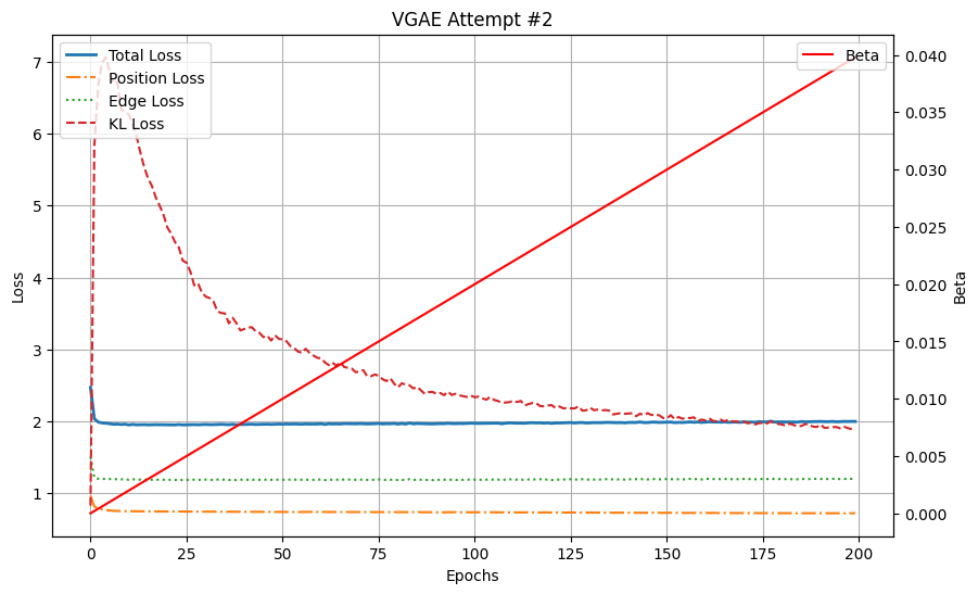
实验 #2:尽管其模型复杂度增加,表现却不如实验 #1。位置损失、边损失和 KL 损失迅速稳定在较高值(分别为 0.72、1.2 和 1.89),表明重建效果不佳。进一步训练仅降低了 KL 损失,而没有改善重建质量。
我们观察到终端位置损失为 0.72,边损失为 1.2,KL 损失为 1.89。
有趣的是,尽管这个模型更复杂,重建误差衰减并迅速稳定,而进一步训练仅用于降低 KL 损失。查看一个重建示例证实我们的模型学习效果不佳—
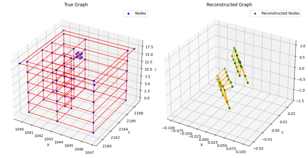
验证样本实验 #2
VGAE 实验 #3:残差 MLP
在这个实验中,我们将从图卷积转向更传统的架构。我们的编码器和解码器将由带有跳跃连接的 MLP 形成的顺序残差块组成。
import torch
import torch.nn as nn
from torch import Tensor
from torch_geometric.nn import GCNConv, InnerProductDecoder
from torch_geometric.utils import negative_sampling

EPS = 1e-15

classResidualBlock(nn.Module):
'''
    A Residual Block for deep neural networks, designed to mitigate the vanishing gradient problem.
    It consists of two fully connected layers with an activation function, with a skip connection
    that adds the input back to the output.'''

def__init__(self, hidden_dim, activation=nn.LeakyReLU, negative_slope=0.2):
super().__init__()
self.fc1 = nn.Linear(hidden_dim, hidden_dim) # First fully connected layer
self.act = activation(negative_slope=negative_slope) # Activation function
self.fc2 = nn.Linear(hidden_dim, hidden_dim) # Second fully connected layer

defforward(self, x):
'''Forward pass of the Residual Block.'''
        residual = x # Save the input for the skip connection
        out = self.fc1(x) #linear
        out = self.act(out) # activation
        out = self.fc2(out) #linear
        out = out + residual #adding the input back to the output through skip connection.It prevents vanishing gradient, a phenomenon often seen with deep nn.
return out

classVGEncoder(nn.Module):
def__init__(self, in_channels=3, out_channels=4):
'''Variational Graph Encoder (VGEncoder) using a sequence of residual blocks.'''
super().__init__()
# Initial fully connected layer with activation
        hidden_dim = out_channels
self.init_fc = nn.Linear(in_channels, hidden_dim)
self.act = nn.LeakyReLU(negative_slope=0.2)

# Sequence of residual blocks
self.res_blocks = nn.Sequential(
            ResidualBlock(hidden_dim),
            ResidualBlock(hidden_dim),
            ResidualBlock(hidden_dim),
            ResidualBlock(hidden_dim),
            ResidualBlock(hidden_dim),
        )

# Linear layers to compute mean and log standard deviation
self.lin_mu = nn.Linear(hidden_dim, hidden_dim)
self.lin_logstd = nn.Linear(hidden_dim, hidden_dim)

defforward(self, x: Tensor, edge_index: Tensor):
# Initial linear transform + activation
        x = self.act(self.init_fc(x))
# Pass through residual blocks
        x = self.res_blocks(x)

# Compute mean and log_std
        mu = self.lin_mu(x)
        log_std = self.lin_logstd(x)
return mu, log_std

classAVGAE(nn.Module):
def__init__(self, in_channels=3, hidden_channels=4, out_channels=3):
super().__init__()
self.enc = VGEncoder(in_channels=in_channels, out_channels=hidden_channels)
self.adj_dec = InnerProductDecoder()
# Position decoder: uses residual blocks similar to the encoder
self.pos_init_fc = nn.Linear(hidden_channels, hidden_channels) # Initial linear transformation with activation
self.pos_act = nn.LeakyReLU(negative_slope=0.2)

self.pos_res_blocks = nn.Sequential(
            ResidualBlock(hidden_channels),
            ResidualBlock(hidden_channels),
            ResidualBlock(hidden_channels),
            ResidualBlock(hidden_channels),
            ResidualBlock(hidden_channels),
            ResidualBlock(hidden_channels),
        )

self.pos_final = nn.Linear(hidden_channels, out_channels)

defreparametrize(self, mu: Tensor, logstd: Tensor) -> Tensor:
'''
        Reparameterization trick to sample from a Gaussian distribution.

        Parameters:
        - mu is the mean of the latent distribution.
        - logstd is the Log of the standard deviation of the latent distribution.

        Returns:
        - Sampled latent variable z.
        '''
ifself.training:
return mu + torch.randn_like(logstd) * torch.exp(logstd) # Apply reparameterization during training to allow gradient flow.
else:
return mu # Using the mean for inference.

defkl_loss(self, mu: Tensor, logstd: Tensor) -> Tensor:
'''Computes the Kullback-Leibler (KL) divergence loss.'''
return -0.5 * torch.mean(
            torch.sum(1 + 2 * logstd - mu**2 - logstd.exp()**2, dim=1)
        )

defadj_recon_loss(self, z: Tensor, pos_edge_index: Tensor,
neg_edge_index: Tensor = None) -> Tensor:
'''Computes the reconstruction loss for the adjacency matrix.'''
# Loss for predicting positive edges.
        pos_loss = -torch.log(self.adj_dec(z, pos_edge_index, sigmoid=True) + EPS).mean()

if neg_edge_index is None:
            neg_edge_index = negative_sampling(pos_edge_index, z.size(0))
        neg_loss = -torch.log(1 - self.adj_dec(z, neg_edge_index, sigmoid=True) + EPS).mean() # Loss for predicting negative edges.

return pos_loss + neg_loss

defpos_recon_loss(self, x: Tensor, edge_index: Tensor, z: Tensor) -> Tensor:
'''Computes the reconstruction loss for the node positions.'''
        out = self.pos_act(self.pos_init_fc(z)) # Initial transformation
        out = self.pos_res_blocks(out) # Pass through residual blocks
        out = self.pos_final(out) # Final transformation
return nn.functional.mse_loss(x, out)

defforward(self, x: Tensor, edge_index: Tensor):
        mu, logstd = self.enc(x, edge_index)  # Encode input graph
        z = self.reparametrize(mu, logstd)  # Sample latent variables
return (self.pos_recon_loss(x, edge_index, z),
self.adj_recon_loss(z, edge_index),
self.kl_loss(mu, logstd))
以下是损失曲线:
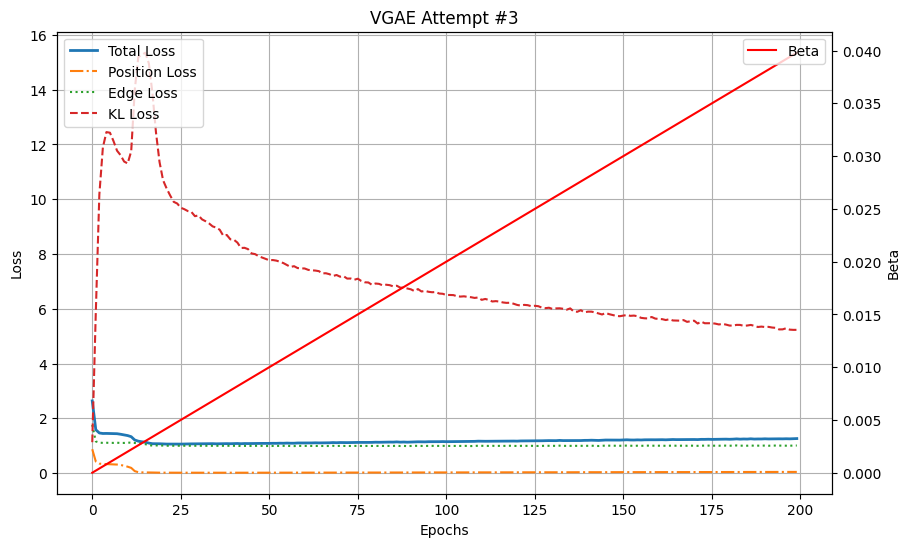
实验 #3 在位置重建方面显示出显著改进,终端位置损失为 0.045,与之前的实验相比有所提高。然而,边缘损失仍然相对较高,为 1.009,KL 损失为 5.320。
首先,终端损失为:位置损失:0.045,边损失:1.009,KL 损失:5.320。位置均方误差显著低于之前。让我们看一个重建示例,
验证样本实验 #3
虽然它显然并不完美,且模型难以学习图的几何结构(例如,许多角度并非正交),但这看起来是朝着正确方向迈出的一步。
请注意,在整个训练过程中,随着 beta 的增加和优化器更侧重 KL 损失,位置重建误差和 KL 损失似乎呈现出反向演变:当其中一个上升时,另一个则下降。在接下来的部分,我们将根据两种不同的退火调度来调整 beta,试图纠正这一问题。
实验 #4:KL 损失的 sigmoidal 调度
我们的第一个调度方案将 beta 根据逻辑调度进行变化。在训练的前 80% 期间,beta 将接近于零,然后迅速上升到大约 0.1。这里的直觉是,我们允许模型尽可能长时间地专注于最小化重建误差,而只在训练的后期专注于 KL 损失。
import datetime
import math
import os
import torch
import torch.nn as nn
import torch.nn.functional as F
from torch.optim.lr_scheduler import StepLR
from torch import Tensor
from torch_geometric.utils import negative_sampling

deftrain(model,
          train_data,
          optimizer,
          scheduler,
          beta_final=0.1,
          num_epochs=5000,
          save_dir="training_checkpoints",
          save_every=100):

# Create a timestamped directory for this training run
    timestamp = datetime.datetime.now().strftime("%Y%m%d_%H%M%S")
    run_dir = os.path.join(save_dir, f"run_{timestamp}")
    os.makedirs(run_dir, exist_ok=True)

print(f"Model checkpoints and logs will be saved to: {run_dir}")

    model.train()
if torch.cuda.is_available():
        model.cuda()

    losses = []
    losses_pos = []
    losses_adj = []
    losses_kl = []
    betas = []

# Parameters for beta schedule
    center = 0.8# The fraction of training after which beta starts to rise steeply
    sharpness = 10.0# Controls steepness of transition

for epoch inrange(num_epochs):
# Compute progress ratio
        progress = epoch / num_epochs
# Beta schedule using logistic growth:
# Before ~80% of training, beta ~ 0; after that, it rises sharply towards beta_final
        beta = beta_final * (1.0 / (1.0 + math.exp(-sharpness * (progress - center))))

        epoch_loss = 0
        epoch_pos_loss = 0
        epoch_adj_loss = 0
        epoch_kl_loss = 0

for sample in train_data:
            x = normalize_features(torch.tensor(sample['building_points'], dtype=torch.float))
            edge_index = sample['building_adj_matrix']

if torch.cuda.is_available():
                x = x.cuda()
                edge_index = edge_index.cuda()

            optimizer.zero_grad()

# Forward pass
            loss_pos, loss_adj, loss_kl = model(x, edge_index)
            loss = loss_pos + loss_adj + beta * loss_kl

# Backward pass
            loss.backward()
            optimizer.step()

# Update epoch loss
            epoch_loss += loss.item()
            epoch_pos_loss += loss_pos.item()
            epoch_adj_loss += loss_adj.item()
            epoch_kl_loss += loss_kl.item()

        scheduler.step()

        avg_loss = epoch_loss / len(train_data)
        avg_kl_loss = epoch_kl_loss / len(train_data)
        avg_position_loss = epoch_pos_loss / len(train_data)
        avg_edge_loss = epoch_adj_loss / len(train_data)

        losses.append(avg_loss)
        losses_kl.append(avg_kl_loss)
        losses_pos.append(avg_position_loss)
        losses_adj.append(avg_edge_loss)
        betas.append(beta)

print(f"Epoch {epoch + 1:04d}, Beta: {beta:.4f}, Total Loss: {avg_loss:.4f}, KL Loss: {avg_kl_loss:.4f}, Position Loss: {avg_position_loss:.4f}, Edge Loss: {avg_edge_loss:.4f}")

# Save checkpoint every save_every epochs
if (epoch + 1) % save_every == 0or (epoch + 1) == num_epochs:
            checkpoint_path = os.path.join(run_dir, f"model_epoch_{epoch+1}.pt")
            torch.save({
'epoch': epoch + 1,
'model_state_dict': model.state_dict(),
'optimizer_state_dict': optimizer.state_dict(),
'losses': losses,
'losses_kl': losses_kl,
'losses_pos': losses_pos,
'losses_adj': losses_adj,
'betas': betas
            }, checkpoint_path)
print(f"Checkpoint saved to {checkpoint_path}")

print(f"Training completed. Model and logs saved in: {run_dir}")

return model, losses, losses_kl, losses_pos, losses_adj, betas

model = AVGAE()
print(f"{torch.cuda.is_available()=}")
optimizer = torch.optim.Adam(model.parameters(), lr=1e-3)
scheduler = StepLR(optimizer, step_size=1000, gamma=0.1)
trained_model, total_losses, kl_losses, position_losses, edge_losses, betas = train(
    model,
    train_data,
    optimizer,
    scheduler,
    beta_final=0.1,
    num_epochs=200,
    save_every=100
)
实验 #4 导致了更高的终端位置重建误差 0.09,这表明与之前的实验相比,重建质量有所下降。虽然 sigmoidal 调度在初期抑制了 KL 损失,但随着 beta 在训练后期增加,早期训练中实现的重建收益被丢失了。这表明 beta 的急剧变化可能扰乱了模型优化。
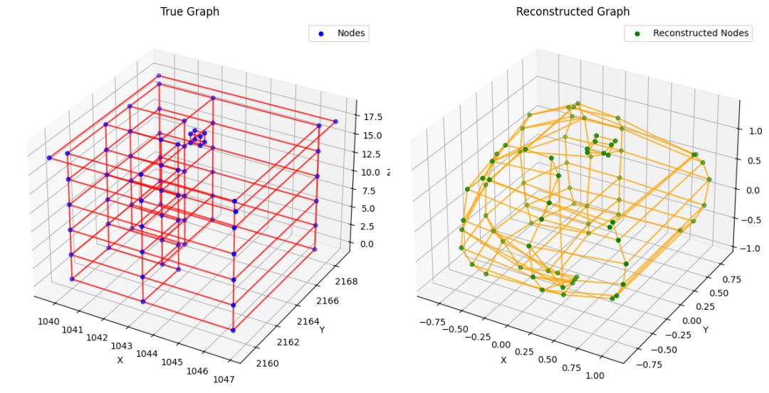
验证样本实验 #4
终端位置重建误差更高,达到 0.09。不幸的是,我们在训练初期通过抑制 KL 损失所看到的重建增益,在训练结束时已经全部丢失。我们的下一个计划将尝试解决这个问题。
计划#2:循环计划
在这里,我们将使用 Fu 等人论文《Cyclical Annealing Schedule: A Simple Approach to Mitigating KL Vanishing》中提出的循环退火计划。
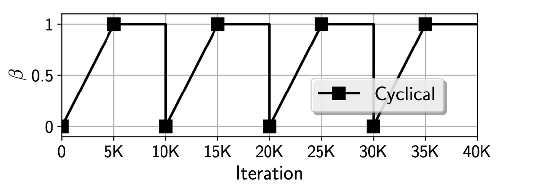
尽管我们的 KL 损失没有消失,但循环计划可能仍然有用:论文认为,在训练初期对 KL 损失赋予高权重(正如本计划所做的那样)可以促使潜在空间早期保持平滑,从而提高解码器的性能。相反,我们初期抑制 KL 损失的 S 形计划可能会让解码器为失败做准备,因为它试图在一个混乱的潜在空间上最小化重建误差。
这是我们的实现:
import datetime
import math
import os
import torch
import torch.nn as nn
import torch.nn.functional as F
from torch.optim.lr_scheduler import StepLR
from torch import Tensor
from torch_geometric.utils import negative_sampling

deftrain(model,
          train_data,
          optimizer,
          scheduler,
          beta_final=1.0,  # According to Fu et al., beta reaches 1 at the peak
          M=4,             # Default number of cycles
          R=0.5,           # Default proportion of increasing phase in each cycle
          num_epochs=5000,
          save_dir="training_checkpoints",
          save_every=100):

# Create a timestamped directory for this training run
    timestamp = datetime.datetime.now().strftime("%Y%m%d_%H%M%S")
    run_dir = os.path.join(save_dir, f"run_{timestamp}")
    os.makedirs(run_dir, exist_ok=True)

print(f"Model checkpoints and logs will be saved to: {run_dir}")

    model.train()
if torch.cuda.is_available():
        model.cuda()

    losses = []
    losses_pos = []
    losses_adj = []
    losses_kl = []
    betas = []

    T = num_epochs
    cycle_length = T / M  # Length of each cycle

for epoch inrange(num_epochs):
# t is the iteration count, starting from 1
        t = epoch + 1

# Compute τ for this iteration:
# τ ∈ [0,1) maps the progress within the current cycle
        tau = ((t - 1) % (cycle_length)) / cycle_length

# Compute beta based on τ:
# If τ ≤ R, increase linearly from 0 to 1
# If τ > R, beta stays at 1
if tau <= R:
            beta = (tau / R) * beta_final
else:
            beta = beta_final

        epoch_loss = 0
        epoch_pos_loss = 0
        epoch_adj_loss = 0
        epoch_kl_loss = 0

for sample in train_data:
            x = normalize_features(torch.tensor(sample['building_points'], dtype=torch.float))
            edge_index = sample['building_adj_matrix']

if torch.cuda.is_available():
                x = x.cuda()
                edge_index = edge_index.cuda()

            optimizer.zero_grad()

# Forward pass
            loss_pos, loss_adj, loss_kl = model(x, edge_index)
            loss = loss_pos + loss_adj + beta * loss_kl

# Backward pass
            loss.backward()
            optimizer.step()

# Update epoch loss
            epoch_loss += loss.item()
            epoch_pos_loss += loss_pos.item()
            epoch_adj_loss += loss_adj.item()
            epoch_kl_loss += loss_kl.item()

        scheduler.step()

        avg_loss = epoch_loss / len(train_data)
        avg_kl_loss = epoch_kl_loss / len(train_data)
        avg_position_loss = epoch_pos_loss / len(train_data)
        avg_edge_loss = epoch_adj_loss / len(train_data)

        losses.append(avg_loss)
        losses_kl.append(avg_kl_loss)
        losses_pos.append(avg_position_loss)
        losses_adj.append(avg_edge_loss)
        betas.append(beta)

print(f"Epoch {epoch + 1:04d}, Beta: {beta:.4f}, Total Loss: {avg_loss:.4f}, KL Loss: {avg_kl_loss:.4f}, Position Loss: {avg_position_loss:.4f}, Edge Loss: {avg_edge_loss:.4f}")

# Save checkpoint every save_every epochs
if (epoch + 1) % save_every == 0or (epoch + 1) == num_epochs:
            checkpoint_path = os.path.join(run_dir, f"model_epoch_{epoch+1}.pt")
            torch.save({
'epoch': epoch + 1,
'model_state_dict': model.state_dict(),
'optimizer_state_dict': optimizer.state_dict(),
'losses': losses,
'losses_kl': losses_kl,
'losses_pos': losses_pos,
'losses_adj': losses_adj,
'betas': betas
            }, checkpoint_path)
print(f"Checkpoint saved to {checkpoint_path}")

print(f"Training completed. Model and logs saved in: {run_dir}")

return model, losses, losses_kl, losses_pos, losses_adj, betas

model = AVGAE()
print(f"{torch.cuda.is_available()=}")
optimizer = torch.optim.Adam(model.parameters(), lr=1e-3)
scheduler = StepLR(optimizer, step_size=1000, gamma=0.1)
trained_model, total_losses, kl_losses, position_losses, edge_losses, betas = train(
    model,
    train_data,
    optimizer,
    scheduler,
    beta_final=1.0,
    M=4,
    R=0.5,
    num_epochs=200,
    save_every=100
)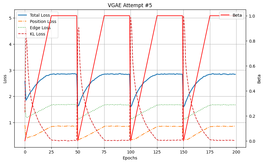
实验 #5:模型在多个周期内保持了重建和正则化之间的平衡。这种策略有助于缓解使用 Sigmoid 调度时出现的问题,即 KL 损失的后期引入会破坏优化。
结论
这些构成了训练用于 3D 建筑生成的图变分自编码器的尝试。在实验中,我们逐步改进了 VGAE 架构和训练策略。实验 1 揭示了模型容量不足以处理数据集的复杂性,因此在实验 2 中进行了调整,如更深的 GCN 层和增加隐藏维度,尽管结果恶化。实验 3 引入了残差 MLP,改善了位置重建但几何精度问题仍然存在,而实验 4 探索了 beta 调度以平衡 KL 损失和重建损失,显示出潜力但需要进一步优化。
图 VAE 是一种训练难度较大的模型,存在 KL 散度收敛问题的可能性。由于任务的复杂性、与传统图分子研究的差异以及训练 GVAE 的固有复杂性,该项目过程中出现了许多瓶颈。
参考文献
[1] World Green Building Council. Bringing Embodied Carbon Upfront. 2019 Publication.
[2] Kipf Thomas, Max Welling. Variational graph auto-encoders. 2016. arXiv:1611.07308.


内容中包含的图片若涉及版权问题,请及时与我们联系删除
评论
沙发等你来抢